7 Flow, cuts, matching
One must step back to leap better.
French proverb, Dictionnaire de l’Académie française (1694)
An hour saved at a non-bottleneck is a mirage.
Eliyahu M. Goldratt and Jeff Cox, The Goal (1984)
7.1 Moving day
Saturday, 8 a.m. A hired van backs up to the curb. Four friends, Juan, Anita, Daniel and Tomás, are moving into one flat together, and they have the van and one car. Juan signed the lease and planned the day, and only Juan has seen the building.
The first question of the day is where the boxes go. Everything in the van has to get up to the flat, through a building with a front door and a lift, a courtyard gate and back stairs.
Another question waits for the evening. The four friends will share the flat’s four rooms, and only two of the rooms face the quiet courtyard. Who gets the quiet rooms?
There is also a question about the friends’ old flats. Someone has to collect each friend’s things, with the van or with the car. The van can carry three loads, and the car can carry one. Collecting takes more effort from some flats than from others. Which vehicle should collect whose things?
The last question is the rent, which is 2,000 euros a month. The friends do not value the rooms alike. Who takes which room, and how is the rent split so that nobody would rather have someone else’s room at that room’s share?
Each of the four questions asks for the best plan for one scarce thing: the ways up, the quiet rooms, the space in the vehicles and the rent. The chapter meets the questions in this order.
Behind all four questions stands one difficulty. A plan can look fine and still be beaten by a better plan that nobody thought of. So far, none of the four friends knows how to tell whether a better plan exists. For the boxes, the van is hired by the hour, so nobody can afford to start over.
A plan that looks fine has already arrived. Daniel’s message in the group chat reads, “plan: everything through the front, along the corridor, up the back stairs, the lift is too slow.” But Daniel has never seen the building. Only Juan has, so only Juan can check whether the boxes can go that way.
7.2 Daniel’s plan is stuck
Networks and maximum flow
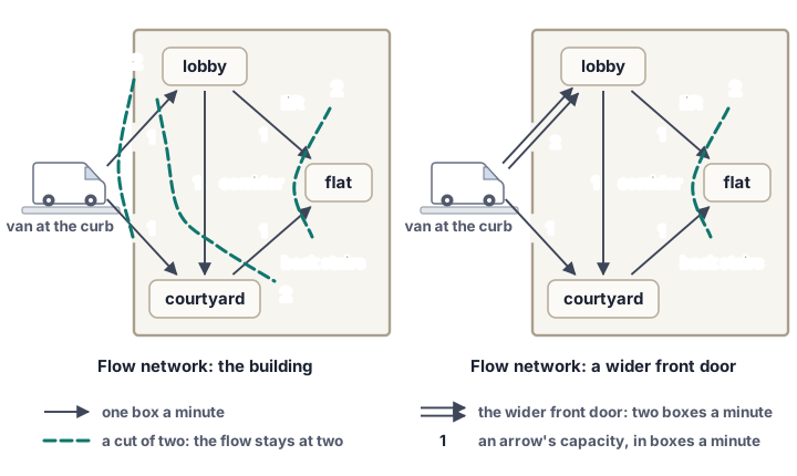
Juan reads Daniel’s message against the building, which has four places: the van at the curb, the lobby, the courtyard and the flat. Five passages connect them. Each passage runs in one direction only and takes at most one box a minute. Daniel’s plan sends everything through the front door, along the corridor and up the back stairs (Figure 7.1).
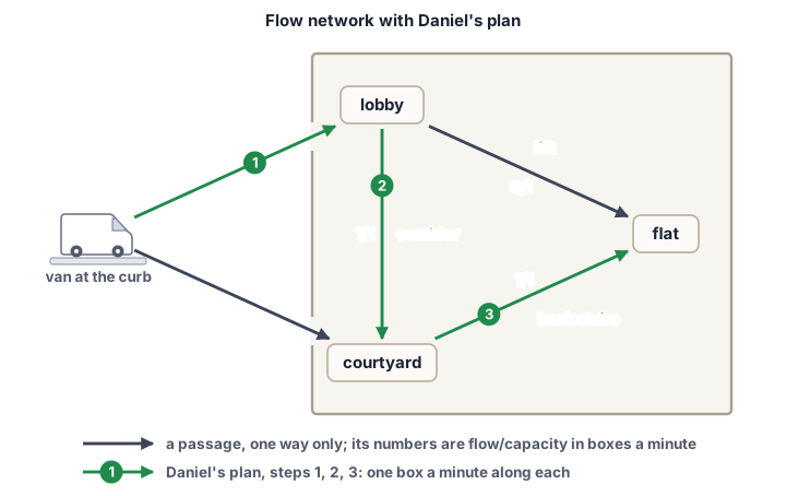
Someone has already sent one box a minute along the front door, the corridor and the back stairs (Figure 7.1). Can you improve the plan, and say why no plan does better?
Three minutes. You’re done when you have a number and a reason, or a move you would undo.
As in the graphs chapter, each place is a vertex of a graph, and each passage is an arrow, a one-way connection. From the van, the front door leads into the lobby, and the courtyard gate leads into the courtyard. The corridor runs from the lobby to the courtyard. The lift leads from the lobby up to the flat, and the back stairs lead from the courtyard up to the flat.
Daniel’s route is a path, as in chapter 5. The source is the vertex that sends everything, here the van. The sink is the vertex that receives everything, here the flat. The capacity of an arrow is the most that it can carry, here one box a minute. A capacity is a rate, and a plan is a set of rates. Boxes that are already upstairs stay there, so a change of plan changes only where the next boxes go.
A flow network is a directed graph with a capacity on every arrow, a source and a sink. Drawn this way, the building is a flow network.
A flow says how much goes along each arrow. No arrow carries more than its capacity or less than zero. At every vertex other than the source and the sink, what comes in goes out. This is called conservation, the rule that a junction of wires obeys in physics (Kirchhoff’s current law). Daniel’s plan is a flow with one box a minute on the front door, the corridor and the back stairs. The lobby and the courtyard each pass on all that they receive.
The flow amount is what leaves the source, minus what comes back into it. No arrow leads into the van or out of the flat, so here the amount is what leaves the van, and by conservation it is also what reaches the flat. A maximum flow has the largest amount that the network allows. Daniel’s flow has an amount of one box a minute. Is it a maximum flow?
Key idea: flow networks and flows
A flow network is a directed graph with a source, a sink and a capacity \(\ge 0\) on every arrow. A flow puts between zero and the capacity on each arrow. At every vertex other than the source and the sink, what comes in goes out (conservation). The flow amount is what leaves the source, minus what comes back into the source.
In the figures, an arrow shows flow/capacity when a flow is drawn, its capacity alone when none is, and its residual capacity in a residual graph.
Can more be sent? From the van, only the courtyard gate can take one more box, but the only arrow out of the courtyard is the back stairs, which are full. The lift can take one more box too, but the only arrow into the lobby is the front door, which is full. So no path from the van to the flat can take one more box.
Yet a flow of two boxes a minute fits. Juan’s flow sends one box a minute through the front door and up the lift, and one box a minute through the courtyard gate and up the back stairs (Figure 7.2). The corridor carries nothing.
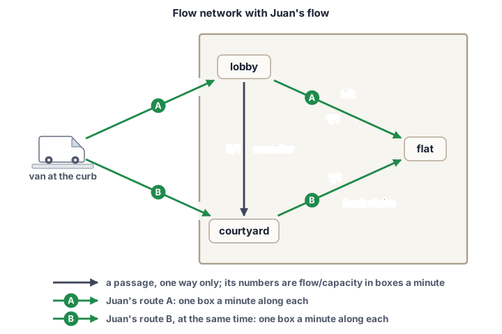
A flow is stuck when it is not a maximum flow, yet no path from the source to the sink can carry more on every arrow. Daniel’s flow is stuck at one box a minute.
The intuitive, but naive, way to improve a flow is greedy addition. Find a path where every arrow can take one more box, send flow along it, and repeat. You might believe that repeating this gives the maximum flow.
The belief is false. Why does the intuitive way get stuck at one box a minute? Daniel’s one path took the front door and the back stairs at once, and the corridor joins them. Each of Juan’s two paths needs one of those two arrows. Sending more never undoes and empties the corridor, so its box-flow stays. By flow conservation, that box-flow occupies the front door and the back stairs. So both stay full, and neither of Juan’s paths is realizable. We are stuck!
So the building alone shows that adding flow and never taking any back can stop below the maximum flow.
The design box states the goal, and the idea that the next sections work out, with the six fields of chapter 1.
To reach two boxes a minute, the corridor’s flow has to move to other arrows. In Juan’s words, “No box comes back down. I only change where the next box goes.” The next section shows how to find such a change.
7.2.1 Taking a box back on paper
Daniel’s flow is stuck at one box a minute, and Juan’s change makes it two boxes a minute. How is such a change found? The result must still be a flow, and what is already right should stay.
Along the arrows as drawn, the obvious search finds nothing. Why not just start over? On a large flow network, a fresh start throws away every good choice already made. The move you want changes one chain of arrows and keeps the rest.
A search along the arrows as drawn can only add flow, but Juan’s change must also take the corridor’s box away. So the move needs one new kind of arrow. For every arrow that carries flow, draw a reverse arrow from the arrow’s end back to its start. One box a minute is one unit of flow. The reverse arrow can take back each unit that was sent the other way. A later path from the source to the sink may run along a reverse arrow. Where it does, it cancels part of an earlier choice.
Taking a unit back moves no box. On paper, the corridor’s unit is canceled, so the next box that would have crossed the corridor goes up the lift instead. The corridor’s reverse arrow, from the courtyard to the lobby, is Juan’s undo arrow. Keeping reverse arrows, so that a commitment can be undone later, is the primitive residual state⬢. Chapter 6’s greedy exchange did without residual state. Each of its steps took the choice that looked best, and no later step undid that choice. For spanning trees, an exchange argument made that safe. For flow, a later step must be able to undo an earlier one, because never taking anything back is how Daniel’s flow got stuck.
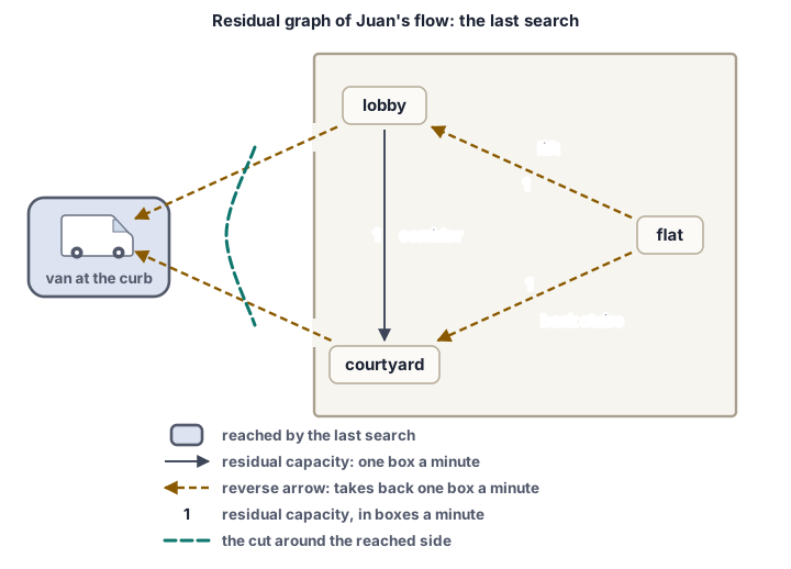
How much an arrow can still carry is its residual capacity [1, Sec. 7.1]. The network’s own arrows are called the forward arrows, and on a forward arrow the residual capacity is the capacity minus the flow. On a reverse arrow, it is the flow that can be taken back. An arrow with residual capacity zero is saturated, and an arrow with residual capacity left is unsaturated. The network redrawn with only its unsaturated arrows is the residual graph.
Figure 7.3 shows the residual graph of Daniel’s flow. The courtyard gate and the lift are unsaturated, so each keeps a residual capacity of one box a minute. The front door, the corridor and the back stairs are saturated, so the residual graph keeps none of them as a forward arrow. In their place, reverse arrows run from the lobby to the van, from the courtyard to the lobby and from the flat to the courtyard. Each can take back one box a minute.
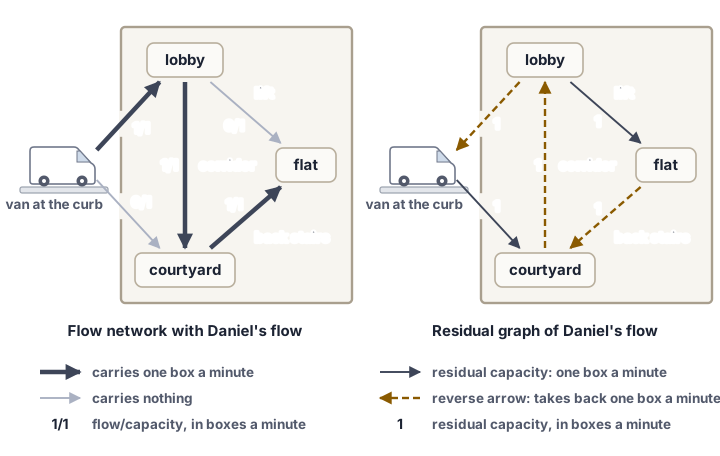
An augmenting path is a path from the source to the sink in the residual graph that visits no vertex twice. It may run along reverse arrows. Juan’s repair path is one. It goes through the courtyard gate, back from the courtyard to the lobby along the corridor’s reverse arrow, and up the lift. On the arrows as drawn, no path can carry more on every arrow. In the residual graph, this one does.
How much can the path send? The bottleneck of an augmenting path is an arrow of the path with the smallest residual capacity. That residual capacity is the most that the path can add to the flow.
Key idea: residual capacity and augmenting paths
Take a flow in a network. The residual capacity of an arrow of the network is its capacity minus its flow. For every arrow that carries flow, a reverse arrow points the other way, and its residual capacity is that flow, the amount that can be taken back. An arrow with residual capacity zero is saturated, and an arrow with residual capacity left is unsaturated. The residual graph has the network’s vertices and every arrow, forward or reverse, whose residual capacity is positive. An augmenting path is a path from the source to the sink in the residual graph that visits no vertex twice. Its bottleneck is an arrow of the path with the smallest residual capacity.
An augmentation sends flow along the augmenting path until its bottleneck is saturated. Every arrow of the path changes by the same amount, the bottleneck’s residual capacity. On each forward arrow of the path, the flow goes up by that amount. On each reverse arrow of the path, the flow on the forward arrow that it reverses goes down by that amount. On Juan’s repair path, every arrow can take one box a minute, so every arrow is a bottleneck, and the amount is one box a minute. The courtyard gate and the lift go up to one box a minute, and the corridor goes back down to zero. The result is Juan’s flow of two boxes a minute (Figure 7.4).
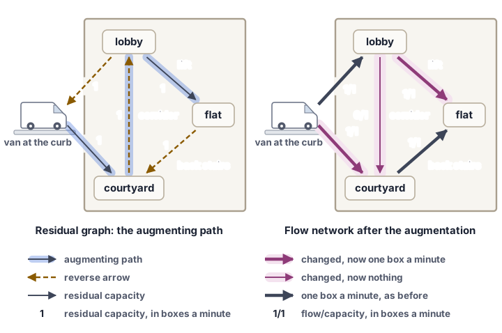
In every network, the result of an augmentation is again a flow [1, p. (7.1)]. Staying within capacity is the easy half. The amount fits within the residual capacity of every arrow on the path, so no arrow goes over its capacity or below zero. Conservation holds for a less obvious reason. Take a vertex inside the path. The path visits it once, so one arrow of the path comes into it, and one goes out. When the path arrives along a reverse arrow, that arrow undoes flow on a forward arrow that leaves the vertex. Four cases cover every vertex inside the path.
- Arriving along a forward arrow raises what comes in by the amount.
- Arriving along a reverse arrow lowers what goes out by the amount.
- Leaving along a forward arrow raises what goes out by the amount.
- Leaving along a reverse arrow lowers what comes in by the amount.
The arrival adds the amount to the difference between what comes in and what goes out, and the departure takes the amount off again. So the difference stays at zero, and what comes in still equals what goes out.
What did one augmentation buy, and at what price? The flow rose by one box a minute, from one box a minute to two boxes a minute. Daniel’s front door and back stairs stayed as they were. The price is one search for every augmentation, because the residual graph changes after each one. After this augmentation, the corridor is unsaturated again, and its reverse arrow is gone. The courtyard gate and the lift now carry flow, so they get reverse arrows. They are saturated, so the residual graph keeps neither of them as a forward arrow.
7.2.2 Again, until no path is left
Ford–Fulkerson method
A run of the Ford–Fulkerson method starts from the zero flow, which sends nothing along any arrow. With nothing sent, there is nothing to take back, so the residual graph is the flow network itself.
Search the residual graph for an augmenting path, augment along it until its bottleneck is saturated, and search again. When a search finds no augmenting path, stop and return the flow. This loop, started from the zero flow, is the Ford–Fulkerson method [2, Sec. 24.2]. Improving a flow along augmenting paths until none is left is a primitive. It is named after the step that it repeats, augmentation⬢.
Start with the building. From the zero flow, Daniel’s route through the front door, the corridor and the back stairs is an augmenting path, and every arrow of it is a bottleneck of one box a minute. So Daniel’s plan was the first augmentation, and Juan’s repair was the second (Figure 7.4). Then the method searches once more. The front door and the courtyard gate are both saturated, so the residual graph has no arrow out of the van. The search finds no augmenting path, and the run stops at two boxes a minute.
In the building, every augmentation sent one box a minute. On the network in Figure 7.5 the amounts differ. The figure draws its eight arrows with their capacities, and the next sentences list them. Four vertices, \(a\), \(b\), \(c\) and \(d\), sit between the source \(s\) and the sink \(t\). The arrows \(s \to a\), \(s \to b\) and \(b \to c\) have capacity 4. The arrows \(a \to b\), \(a \to d\) and \(c \to t\) have capacity 5. The arrows \(c \to d\) and \(d \to t\) have capacity 2. Say the first search finds \(s \to a \to b \to c \to t\). Its bottlenecks are \(s \to a\) and \(b \to c\), with residual capacity 4, so the amount is 4. Now \(s \to a\) is saturated, so the next augmenting path must start with \(s \to b\). It goes from \(b\) back to \(a\) along the reverse arrow of \(a \to b\), and on through \(a \to d\) and \(d \to t\). Its bottleneck is \(d \to t\), with residual capacity 2, so it takes back 2 of the 4 that \(a \to b\) carries, and the amount grows to 6. The third search finds no augmenting path, and the run stops at 6.
The method never says which augmenting path comes next. Whichever path comes, each augmentation turns a flow into another flow. How many augmentations a run needs depends on the paths that it picks. On the six-vertex network, \(s \to a \to d \to t\) followed by \(s \to b \to c \to t\) takes two augmentations. A run that starts with \(s \to b \to c \to d \to t\) takes three.
This open choice, which augmenting path comes next, is the path rule. Each path rule turns the method into one definite algorithm, and those algorithms can differ in speed. The path rule can be swapped for another one that does the same job. Chapter 6 called a part of this kind a swappable part (Figure 6.27).
Both runs stopped when a search found no augmenting path. Is two boxes a minute the maximum flow in the building, and is 6 the maximum flow on the network? The next section answers that question.
7.3 Is two boxes a minute really the maximum?
Cut certificate; max-flow min-cut theorem
Juan’s flow sends two boxes a minute, and the search finds no augmenting path left. Is it a maximum flow, and how would anyone know without trusting whoever computed it?
Stopping alone convinces nobody. Daniel’s plan also stopped, because no path could take one more box on every arrow, and his one-box-a-minute flow was only half of what fits. Listing every plan works only in a problem this small.
Instead, ask for a certificate beside the answer. As in chapter 1, a certificate is a short proof that anyone can check quickly, much faster than solving the problem again. For a flow, the certificate is a bound that no flow can surpass. The bound is proved once and is valid for every flow. The check has two steps: the answer is a flow, and its amount equals the bound. No flow can carry more than that.
The stuck set of the graphs chapter was a certificate too. Kahn’s method stopped with three people still waiting, and anyone could follow the arrows between them to find the circle.
A certificate gives anyone trustless confidence in the answer, because the answer can be verified independently of who computed it: a person, a library or an AI. The price is a bit of extra work. You already find the answer, and you have to find the bound as well. For a flow, the bound is the tightest cutting line through the building.
7.3.1 A line through the building
What evidence would show that no flow in the building carries more than two boxes a minute, including the flows that nobody has tried?
The obvious evidence is a single slow arrow, and the building has none. Every arrow takes at most one box a minute, yet two boxes a minute reach the flat. One arrow limits only the paths through it, and other paths go around it. So the evidence must be a set of arrows that every path from the source to the sink uses.
Key idea: cuts with a source and a sink
A cut splits the vertices of a flow network into two sides: the source’s side \(S\), which includes the source, and the sink’s side \(T\), which includes the sink. The capacity of a cut is the sum of the capacities of the arrows that cross from \(S\) to \(T\). Arrows that go back from \(T\) into \(S\) do not count.
In the building, a cut is a line with the van on one side and the flat on the other. Figure 7.6 draws all four cuts, C1 to C4. Take C2, with \(S\) = {van, courtyard}. The front door and the back stairs cross from \(S\) to \(T\), so C2’s capacity is two boxes a minute. The corridor goes back into the courtyard, so it does not count.
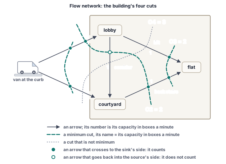
A minimum cut is a cut whose capacity is the smallest of all cuts. The cuts can be listed without drawing. \(S\) always includes the van, and it may include the lobby, the courtyard, both or neither. These four choices give the four cuts (Table 7.1).
| cut | source’s side \(S\) | sink’s side \(T\) | arrows from \(S\) to \(T\) | capacity (boxes a minute) |
|---|---|---|---|---|
| C1 | {van} | {lobby, courtyard, flat} | front door, courtyard gate | 2 |
| C2 | {van, courtyard} | {lobby, flat} | front door, back stairs | 2 |
| C3 | {van, lobby, courtyard} | {flat} | lift, back stairs | 2 |
| C4 | {van, lobby} | {courtyard, flat} | courtyard gate, corridor, lift | 3 |
Why does no flow exceed any cut? By conservation, everything that the source sends must cross every cut to reach the sink. So no flow exceeds any cut, even the narrowest one.
Treat \(S\) as one big vertex. The source inside it sends out the flow amount. Every other vertex inside only passes flow on, by conservation. An arrow with both ends inside moves flow from one inside vertex to another, so that flow never leaves the big vertex.
So the amount must leave the big vertex across the cut. It is what crosses from \(S\) to \(T\) minus what goes back from \(T\) to \(S\). What crosses is at most the cut’s capacity, and what goes back is at least 0:
\[ \begin{aligned} \text{flow amount} &= \text{flow from } S \text{ to } T\\ &\quad {}- \text{flow from } T \text{ to } S\\ &\le \text{capacity of the cut} - 0. \end{aligned} \]
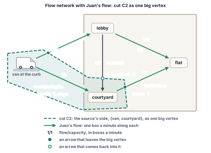
Daniel’s old flow of one box a minute used the front door, the corridor and the back stairs. Across C2, his box leaves, comes back and leaves again. That is \(1 - 1 + 1 = 1\) box a minute, his amount.
So the building has three minimum cuts of two boxes a minute, and none of them is a single slow arrow. No flow exceeds any cut, so no flow carries more than two boxes a minute.
Anyone can check a cut with a few additions, and it bounds every flow at once. But a cut is only a ceiling. It proves that a flow is a maximum flow only when the flow amount equals the cut’s capacity. C4 has a capacity of three boxes a minute, so it proves nothing about Juan’s flow of two boxes a minute.
Does every network have a cut whose capacity equals a maximum flow amount, and how is it found? Trying every cut is as hopeless as trying every flow. Each vertex other than the source and the sink can sit on either side, so a network with 30 vertices has \(2^{28}\) cuts, about 268 million. The next subsection answers both questions.
7.3.2 The line the last search finds
Every run of the Ford–Fulkerson method so far stopped because its last search from the source found no augmenting path (Section 7.2.2). That search followed every arrow of the residual graph that still had residual capacity, forward arrows and reverse arrows alike. As in chapter 5, the source reaches a vertex when a path of such arrows leads from the source to it.
The stopped run hands over its own proof. When no augmenting path is left, the vertices that the last search reaches form the source’s side \(S\) of a cut, and the capacity of this cut equals the flow amount. It is a cut because the source is in \(S\), where the search starts, and the sink is not. A path to the sink would be an augmenting path, and the search found none.
After Juan’s flow of two boxes a minute, the front door and the courtyard gate are both full. The only arrows at the van that still have residual capacity are the two reverse arrows, and they point into the van. So the last search reaches only the van. Its cut is the line through the front door and the courtyard gate. This is C1, one of the three minimum cuts in Figure 7.6. The capacity of this line is two boxes a minute, the same as the amount of Juan’s flow.
On the six-vertex network of Section 7.2.2, the last search reaches \(s\), \(a\), \(b\) and \(d\). The arrows \(b \to c\) and \(d \to t\) cross from \(S\) to \(T\), so the cut’s capacity is 4 + 2 = 6, the amount of the final flow. Figure 7.9 shows this cut.
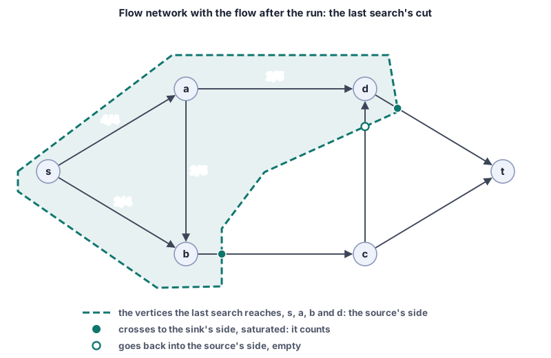
Why must the two numbers agree? The rest of the vertices form the sink’s side \(T\). Treat \(S\) as one big vertex, as in Section 7.3.1. Then
\[ \begin{aligned} \text{flow amount} &= \text{flow from } S \text{ to } T\\ &\quad {}- \text{flow from } T \text{ to } S\\ &= \text{capacity of the cut} - 0. \end{aligned} \tag{7.1}\]
In equation (7.1), every arrow from \(S\) to \(T\) is saturated, and every arrow from \(T\) to \(S\) is empty. Both facts come from where the search stopped. An arrow from \(S\) to \(T\) with residual capacity would have taken the search one vertex further. An arrow from \(T\) to \(S\) that carries flow has a reverse arrow from \(S\) to \(T\) with residual capacity, and the search would have crossed that arrow too. So the second fact needs the reverse arrows of Section 7.2.1.
On Daniel’s flow, a search that ignores reverse arrows crosses the courtyard gate and stops at the courtyard. Two boxes a minute leave that side, but the corridor brings one back in, so the amount is 2 − 1 = 1 box a minute, while the line’s capacity is two boxes a minute. A search that also takes reverse arrows continues along the corridor’s reverse arrow to the lobby.
Ford–Fulkerson stops with a final flow. No flow exceeds the last search’s cut (Section 7.3.1), and the amount of the final flow equals the cut’s capacity. So the final flow is a maximum flow. Every cut’s capacity is at least that amount, and the last search’s cut has exactly that capacity. So it is a minimum cut. This argument holds for every path rule, because it uses only the final flow and the last search.
In its general form, this result is the max-flow min-cut theorem of Ford and Fulkerson [1, Sec. 7.2]. It says that in every flow network, the largest amount of any flow equals the smallest capacity of any cut. In symbols,
\[ \max_{\text{flows}} \text{amount of the flow} = \min_{\text{cuts}} \text{capacity of the cut}. \tag{7.2}\]
A cut whose capacity equals a flow amount is a certificate that anyone can check. This is the primitive cut certifies flow⬢.
So Juan’s flow of two boxes a minute is a maximum flow. The front door and the courtyard gate prove it. Anyone can check this by adding their two capacities, without trying a single other plan.
With integer capacities, every residual capacity starts as an integer. Each augmentation changes the arrows of its path by the bottleneck’s residual capacity, an integer, so every residual capacity stays an integer, and so does the flow on every arrow. This property is called integrality.
The Cost line of the Max flow design box (The design 7.1) also speaks of path rules that take the fewest arrows first. Fewest arrows is chapter 6’s measure for a path. Breadth-first search finds a path with the fewest arrows, and the bound for these path rules comes in Section 7.4.2.
The invariants of the Max flow design box (The design 7.1) are the statements that every augmentation keeps true. Where does the guarantee come from? The first two invariants make the answer a flow, and the cut from the last search proves that this flow is the largest. Integer capacities make every augmentation add at least one unit of flow to the amount. No flow exceeds any cut, so the amount never passes a cut’s capacity. The number of augmentations is therefore at most that capacity, and a run on integer capacities must stop. The next section returns to this count and shows that the path rule sets the cost.
The cut of equal capacity proves that the amount is the largest. It does not prove the speed, which belongs to the path rule, the subject of the next section. It also does not prove that a flow with costs is the cheapest one. That needs a different certificate. Its numbers are heights, and they arrive in Section 7.6.2.
The Max flow box’s Promise is something you can demand of any max-flow code, including code that an AI wrote. Ask for the cut beside the flow, and check that the capacities of the arrows that leave the source’s side add up to the flow amount. The library returns the cut with every answer. You can also choose which path rule runs, as Section 7.4.1 shows.
7.3.3 Where does investing in capacity pay off?
The cut names arrows, not only a number, so it can say where a better building would help. Widening an arrow means raising its capacity. Every minimum cut holds the flow to its capacity. So the flow rises only when every minimum cut gets wider, that is, when each of them has a widened arrow.
The building has three minimum cuts, C1 to C3 (Table 7.1), and its arrows fall into three kinds (Table 7.2).
| widened arrows | in the building | effect |
|---|---|---|
| no arrow in any minimum cut | the corridor | futile alone |
| a set that misses some minimum cut | the front door alone; the front door and the courtyard gate (C3 missed) | the flow stays at two boxes a minute |
| a set with an arrow in every minimum cut | the front door and the back stairs; the front door and the lift; the courtyard gate and the back stairs; a new arrow from the van to the flat | the flow rises |
The corridor is in no minimum cut. Which change to other arrows puts it into the only minimum cut?
Five minutes, with the cut table. You’re done when you have the change and the new minimum cut.
Widening other arrows can move the minimum cuts. Widen the front door and the back stairs to three boxes a minute each, and C4 becomes the only minimum cut. C4 crosses the corridor, so widening the corridor then helps.
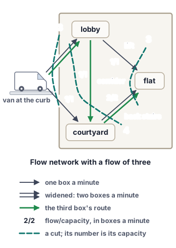
A wider front door alone leaves the flow at two boxes a minute, because C3 does not include it (Figure 7.10). Widen the back stairs as well, and every minimum cut gets wider. The flow rises to three boxes a minute, and the third box goes through the front door, the corridor and the back stairs (Figure 7.11). A whole route from the van to the flat always pays off, because every route crosses every cut.
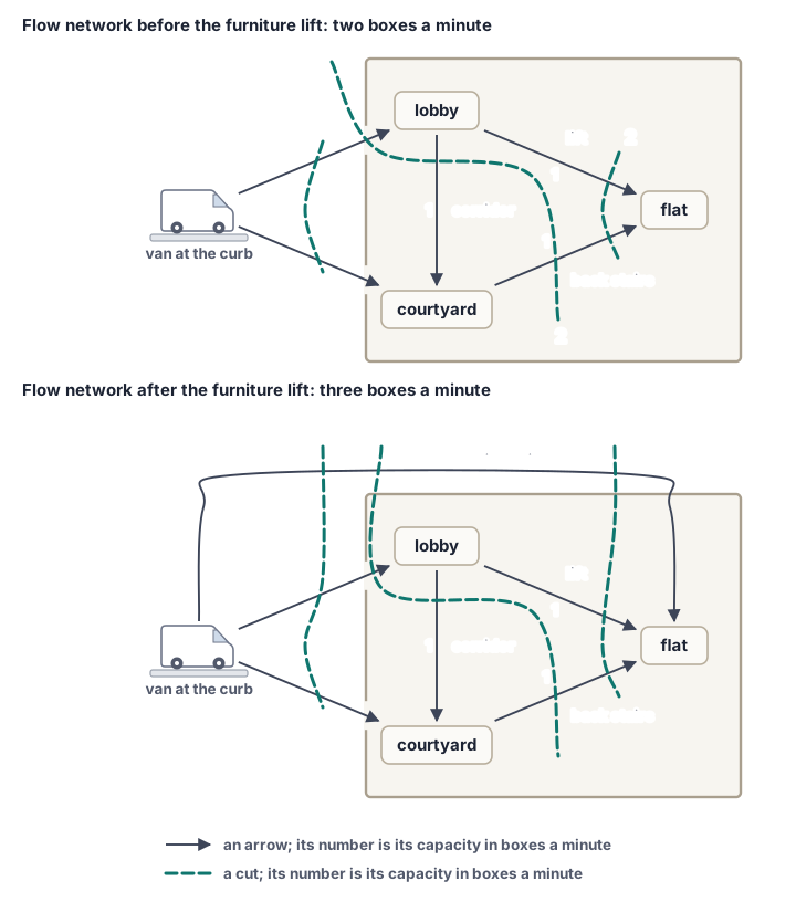
One possible change is a new arrow straight from the van to the flat. A furniture lift through the window is that arrow. It carries one box a minute, and the flow rises to three boxes a minute. It crosses all three minimum cuts, so each of them grows to three boxes a minute (Figure 7.12).
7.4 How long will it take?
One augmentation freed Daniel’s stuck flow. Does every run end at a maximum flow, and after how many augmentations? Each augmentation searches the residual graph, looking at each arrow at most once, and updates one path, so its time is in proportion to the flow network’s size. So a run’s time comes down to the number of augmentations. A good bound on that number uses the network’s size, not the capacities.
A run that stops has no augmenting path left, so it holds a maximum flow (Section 7.3.2). With integer capacities, each augmentation adds at least one unit to the amount. The amount cannot pass a cut’s capacity, so such a run always stops. The amount is a monovariant, a number that moves only one way. How many augmentations does a run need? Taking the path with the fewest arrows bounds the count by the network’s size alone.
The section ends in an open choice, because the path rule is a swappable part, as in chapter 6. Several methods share one loop and differ only in how they choose the paths. So the method is split into two parts:
- a loop that repeats rounds until no augmenting path is left;
- a path rule that, in each round, picks the paths along which the loop augments.
The code keeps the two parts apart, and so do the proofs. The loop and its correctness proof are written once. A path rule runs inside the loop’s code. If it keeps three promises to the loop, the loop’s correctness proof covers it too (Section 7.4.1). Each path rule proves its own speed bound and needs its own code (Section 7.4.4).
7.4.1 One loop, one open choice
The loop is the Ford–Fulkerson method. It augments until no augmenting path is left. The path rule is the one choice that the method leaves open: the paths along which the loop augments. In each round, the loop calls the path rule once. The rule adds along one path or along several paths, or it reports that no augmenting path is left.
The loop starts from the zero flow and lets the rule get ready, because some path rules carry something between rounds. The loop keeps one residual graph, built from the flow network with the zero flow, and hands it to the path rule in every round. The path rule augments it in place, so the flow lives there: the flow on an arrow is the residual capacity of its reverse arrow. Then the loop asks for rounds until a round returns an empty list of paths, which means that no augmenting path is left. Finally the loop returns the flow and a cut, whose source’s side \(S\) holds the vertices that the source still reaches in the residual graph. Here it is in code, from max_flow.py.
The loop ends at a maximum flow if the path rule keeps three promises. First, it adds only along augmenting paths. Each path must still be augmenting after the flow has been added along the round’s earlier paths. The amount that the rule sends along a path must be at most its bottleneck’s residual capacity. Second, with integer capacities, every round that returns a path raises the flow amount by at least one unit. Third, it reports that no augmenting path is left only when none is left.
You state these promises when you ask an AI, or anyone, for a path rule. Any path rule that keeps them is correct, by the proof below. Speed requirements and choosing among path rules come in Section 7.4.4.
By the first promise, the loop holds a flow after every round. By the second, the amount rises by at least one unit per round but cannot pass a cut’s capacity, so the loop stops after finitely many rounds (Section 7.4). By the third, it stops only when no augmenting path is left, and then its cut’s capacity equals the amount, so the flow is a maximum flow (Section 7.3.2).
So every path rule that keeps the three promises ends with a maximum flow and its cut, and one proof covers them all. What each path rule still has to prove is its speed.
7.4.2 Fewest arrows first
With integer capacities, every run ends. The maximum amount bounds the number of augmentations, and that amount depends on the capacities, not on the flow network’s size (Section 7.4). Can the network’s size alone bound how many augmentations a run takes? The Cost line of the Max flow design box (The design 7.1) says yes for path rules that take the fewest arrows first.
Call the next network the 1-and-1000 network. Besides the source and the sink, it has vertices \(a\) and \(b\). Arrows of capacity 1000 run from the source to each of them and from each of them to the sink. The middle arrow goes from \(a\) to \(b\) and has capacity 1.
Take two path rules. The first rule always crosses the middle arrow. It alternates between two paths. One goes from the source through \(a\) and \(b\) to the sink. The other goes from the source through \(b\) and \(a\) to the sink, and its step from \(b\) to \(a\) runs back along the middle arrow’s reverse arrow. The second rule takes an augmenting path with the fewest arrows. How many augmentations does each path rule need?
Two minutes, by reasoning, not by tracing. You’re done when you have both counts.
Any augmenting path gives a correct answer, but not always a quick one. The first rule’s first path crosses the middle arrow, so it adds only 1 unit and fills the middle arrow. The second path goes back along the middle arrow’s reverse arrow, which holds just that 1 unit, so it also adds 1 unit. Each later pair repeats this, so the maximum of 2,000 units takes 2,000 augmentations, where two would be enough (Figure 7.13).
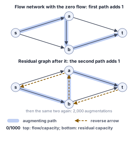
With a million in place of each 1000, the same rule takes two million augmentations on the same five arrows. The count follows the capacities, not the network’s size.
The better rule takes the path with the fewest arrows, which the breadth-first search of Section 6.2.1 finds. Its first-in-first-out queue takes the vertices out in order of their distance from the source, counted in arrows. So the first path that reaches the sink has the fewest arrows.
The Ford–Fulkerson method that always augments along a path with the fewest arrows is the Edmonds–Karp algorithm [2, Sec. 24.2]. Its path rule runs inside the loop of Section 7.4.1.
Edmonds–Karp’s round is one breadth-first search in the residual graph over arrows with at least one unit of residual capacity. If the search reaches the sink, the path rule adds along the path with the fewest arrows, and otherwise it reports that none is left. Here it is in code, from edmonds_karp.py.
Edmonds–Karp’s round calls this search and this augmentation, from edmonds_karp.py and residual.py.
Edmonds–Karp keeps the three promises. Its search uses only arrows with residual capacity, so each of its paths is augmenting and adds at least one unit. Residual capacities stay integers, so every arrow that the search skips is saturated. When the search does not reach the sink, no augmenting path is left. Its correctness comes from the loop, so only its running time needs its own proof. That proof is harder than the proof of correctness.
On the 1-and-1000 network, the search first finds the path from the source through \(a\) to the sink, and then the path through \(b\). Each has two arrows, one fewer than a path across the middle arrow. The two share no arrow, so two augmentations of 1000 reach the maximum.
As in Key idea: graphs, \(n\) counts the vertices, and \(m\) counts the arrows. Edmonds–Karp takes at most about \(nm\) augmentations, whatever the capacities. On the 1-and-1000 network, \(n = 4\) and \(m = 5\), so the bound allows about 20 augmentations, not 2,000.
A vertex’s distance \(d(v)\) is the fewest arrows on a path to it from the source in the residual graph. Each augmentation changes the residual graph: an arrow that fills drops out, and reverse arrows appear. So distances can change. The proof rests on a surprising fact, taken here as given [2], Lemma 24.7: no augmentation brings a vertex closer to the source.
Take an arrow from \(u\) to \(v\) that an augmentation fills. Its path had the fewest arrows, so \(d(v) = d(u) + 1\) at that moment. The arrow can fill again only after a later path takes its reverse arrow, from \(v\) to \(u\). Write \(d'\) for the distances at that later moment. Then
\[ d'(u) = d'(v) + 1 \ge d(v) + 1 = d(u) + 2, \tag{7.3}\]
where the inequality is the fact above. So between two fills of the arrow, \(d(u)\) grows by at least 2. No distance exceeds \(n\), so each residual arrow fills at most about \(n/2\) times. Every augmentation fills at least one of the at most \(2m\) residual arrows, so
\[ \text{augmentations} \le 2m \cdot \frac{n}{2} = nm. \tag{7.4}\]
Each augmentation is one breadth-first search over at most \(2m\) arrows. So the Edmonds–Karp algorithm does \(O(nm^2)\) work in all. The price is a new search for every path, thrown away after one augmentation, although the next path often has just as few arrows. Whether a better path rule can reuse that search is the question of Section 7.4.3.
7.4.3 A whole round of fewest-arrow paths
Edmonds–Karp searches again from the start after every path (Section 7.4.2). Yet one path changes only its own arrows, so most of what the search found still holds. Dinic’s algorithm uses one search for a whole round of paths.
Each round starts with one breadth-first search from the source. It sorts the vertices into layers by the fewest arrows on a path from the source. Layer 0 holds the source alone, layer 1 holds the vertices one arrow away, and so on. The round keeps only the unsaturated arrows that go exactly one layer deeper. So every path of kept arrows from the source to the sink has the fewest arrows.
The round then sends flow along such paths, one after another, until each of them has a saturated arrow. A depth-first walk finds them, and an arrow that has led to a dead end is not tried again in that round. When the round ends, every path with this round’s number of arrows has a saturated arrow. The round’s new reverse arrows point one layer back, so when the next round searches again, the sink lies at least one layer deeper. The run stops when a search no longer reaches the sink. Step through the rounds in Figure 7.14.
Dinic’s algorithm is the loop with this path rule, so it is correct for the same reason as Edmonds–Karp. The sink can move deeper at most \(n\) times, so a run has at most \(n\) rounds. In one round, each path takes about \(n\) steps and fills at least one kept arrow, so a round sends along at most \(m\) paths. Each dead end is tried once, so a round takes \(O(nm)\) steps. So the bound is \(O(n^2 m)\) steps, whatever the capacities. That beats Edmonds–Karp’s \(O(nm^2)\) when arrows outnumber vertices. Dinic’s rule is the library’s default (dinic.py).
7.4.4 Trading code for speed
Edmonds–Karp and Dinic both have bounds that depend only on \(n\) and \(m\), but both take far fewer steps than their bounds allow. So only measurement can say whether Dinic’s extra code pays. Two things are measured: lines of code and running time. The path rules ran on a measured mix of 18 generated flow networks of several kinds, from networks that pair people with objects to long, thin networks.
A third path rule joins Edmonds–Karp and Dinic. Capacity scaling uses only augmenting paths whose arrows all have at least a threshold of residual capacity. The threshold starts at the largest capacity rounded down to a power of two. It halves whenever no such path is left, until it reaches 1. So the big paths go first. Writing this rule is a self-check problem.
Compare the path rules on one network in Figure 7.15. Edmonds–Karp takes four rounds, one path each. Dinic sends the three paths of two arrows in one round. Capacity scaling sends the big paths first and never uses the arrow from \(c\) to \(t\).
Keep a path rule only if no other one beats it on both code and time. The path rules that are left form the Pareto frontier, chapter 1’s picture for designs (Figure 7.16). The frontier bends toward the ideal point, no code and no time. Here all three path rules stay on it.
- Edmonds–Karp has the least code and is the slowest. On average it took about 61 times as long as Dinic.
- Capacity scaling sits between them. On long, thin networks with a wide range of capacities, it took 0.39 to 0.72 of Dinic’s time.
- Dinic has the most code of the three and is the fastest.
A fourth path rule, Dinic with scaling, runs Dinic’s rounds under capacity scaling’s threshold. It has more code than Dinic and took about 2.3 times as long, so Dinic beats it on both measures, and it drops off the frontier.
Push-relabel comes from another family of methods. Its time was about a fifth of Dinic’s, on average over the same 18 networks. Push-relabel has about two and a half times as much code as Dinic (appendix).
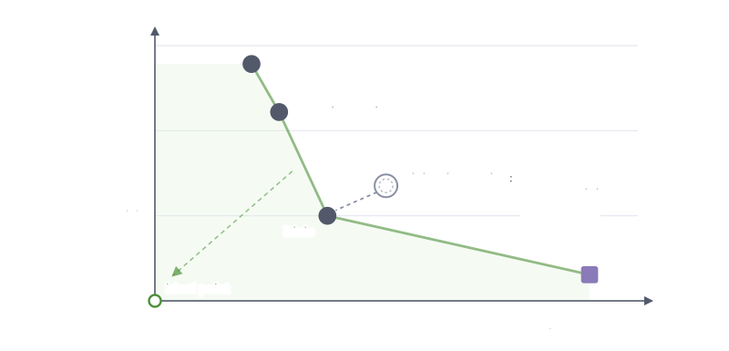
Why does the chapter explain the slowest path rule? The code axis says more than how long a program is. More code usually means more ideas. Each idea is one more thing that a reader must learn. On a Pareto frontier, a preference picks the point. This is a textbook, so our preference is Edmonds–Karp, the path rule that is easiest to explain. Push-relabel is the fastest method here, about 300 times faster than Edmonds–Karp. But it brings ideas of its own. Water pools at a vertex, and the vertex rises until the water can run on. It is harder to explain, so it gets only an appendix. Another situation brings another preference. For production code on large networks, the pick would most likely be push-relabel.
So choose on the frontier by your workload, the networks that you will meet. With no workload in hand, take Dinic, the library’s default. It is the fastest path rule on average over the whole mix, and its bound does not depend on the capacities. The points are one machine’s times on one mix, so measure again where your networks differ. And since the cut checks every answer, a new path rule needs no trust. As with any certificate (Section 7.3), its answers are verified independently of who wrote it, a person or an AI. The certificate checks the answer, not the time. A path rule can return a correct flow and still break its promise on speed.
7.5 Who gets the quiet rooms?
Matchings in bipartite graphs
That evening the boxes are in the flat, and the four friends choose among four rooms. Rooms 1 and 2 face the quiet courtyard, and rooms 3 and 4 face the street. Anita, Daniel and Tomás are light sleepers, so they want a quiet room. Room 2 is next to the noisy lift (elevator), so Anita and Daniel accept only room 1. Tomás accepts room 1 or room 2. He arrived first and took room 1. Juan accepts a street room, room 3 or room 4 (Figure 7.17).
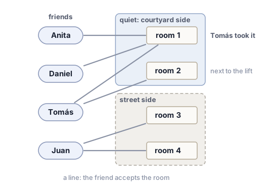
They want as many friends as possible in a room that they accept, with one room per friend and one friend per room.
Give as many friends as possible a room that they accept (Figure 7.17). If not everyone can have one, say who proves it.
Three minutes. You’re done when you name a pairing, or a group of friends that explains who misses out.
The friends and the rooms can be modeled as the vertices of a graph. Each room that a friend accepts gives a link between the two, the two-way link of the graphs chapter. Such a friend and room are an acceptable pair.
A graph whose vertices fall into two sides, with every link joining one side to the other, is a bipartite graph. Here the friends are one side and the rooms are the other.
A set of acceptable pairs in which no person and no object appears twice is a matching. It says who sleeps in which room. Anita in room 1 and Juan in room 3 is a matching. Anita and Daniel both in room 1 is not a matching, because room 1 appears twice. Daniel in room 2 is not a matching either, because he does not accept room 2.
A maximum matching is a matching with as many pairs as any matching can have. Two matchings with the same number of pairs are equally good, even when different friends get room 1. So the friends’ question asks for a maximum matching in this bipartite graph.
Key idea: matchings
A bipartite graph is a graph whose vertices fall into two sides, \(L\) and \(R\), with every link joining a vertex of \(L\) to a vertex of \(R\). A matching is a set of links in which no vertex appears twice. A maximum matching is a matching with as many links as any matching can have. For example, \(L\) can be people, \(R\) objects, and a link an acceptable pair.
Now try the obvious way. Pair the friends one at a time, and never move anyone who already has a room. Tomás keeps room 1, where he already is, and Juan takes room 3. This way gets stuck for Anita and Daniel, and neither gets a room. Each has only one link, and it ends at room 1, which the matching already uses.
Why did this happen? Tomás took room 1 first, and room 1 is the only room that Anita and Daniel accept. But Tomás accepts room 2 as well.
A matching that only grows keeps every pair. So an early pair can take the only object that a later person accepts, and that person is left out. Daniel’s plan kept its box a minute on the corridor in the same way.
Pairing this way never asks whether moving Tomás would let one more friend in.
The Matching design box states the goal, and the idea that the next two sections work out.
7.5.1 Pairing as a flow
Max flow already knows how to take a choice back. Can it also find the largest matching of friends and rooms?
Matchings need no new method. Turning a new problem into one that a known method already solves is a reduction⬢. Chapter 5 turned 2-SAT into a question about paths (Section 5.3.4). Chapter 6 turned the knapsack into a longest path (Section 6.4). Here a matching becomes a flow.
The matching network has a source, a sink, one vertex for every person and one vertex for every object. An arrow of capacity 1 goes from the source to every person. An arrow of capacity 1 goes along every acceptable pair, from the person to the object. An arrow of capacity 1 goes from every object to the sink. Max flow runs on this network. The arrows along the acceptable pairs are the middle arrows, and the middle arrows that carry one unit are a maximum matching. For the flat, four arrows leave the source, six middle arrows follow the acceptable pairs, and four arrows enter the sink (Figure 7.18).
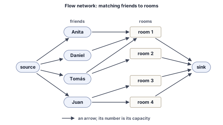
Why is a maximum flow a maximum matching? One unit of flow through a person is that person getting one object. Two facts show that the largest flow and the largest matching have the same size.
- Every matching gives a flow of the same amount. For each pair, send one unit from the source through the person and the object to the sink. No arrow gets more than its capacity of 1, because no person and no object is in two pairs.
- Every integer flow gives a matching of the same size. Each arrow has capacity 1, so an integer flow carries 0 or 1 on it. A person takes in at most one unit, so at most one of the person’s middle arrows carries a unit. An object passes on at most one unit, so at most one middle arrow into it carries a unit. So the middle arrows that carry a unit form a matching, with as many pairs as the flow amount.
Integer capacities don’t make every maximum flow an integer flow. When a person has two objects that serve equally well, half a unit to each can also be a maximum flow, and that is no matching. Integrality guarantees only that an integer maximum flow exists, and every method of this chapter finds one.
So when you need a largest matching, build this network and run any max-flow code that returns an integer flow, as every method of this chapter does.
The reduction is a few lines long. Here it is in code, from matching.py.
Run the method by hand from the stuck matching: Tomás in room 1 and Juan in room 3, a flow of 2 units. Daniel’s only room, room 1, is full. But the residual graph has a reverse arrow from room 1 back to Tomás. So the search goes from the source to Daniel, to room 1, back to Tomás, on to room 2 and to the sink. One unit along this path gives Daniel room 1 and moves Tomás to room 2, so the matching has three pairs. The next search reaches Anita but finds no augmenting path, and the run stops.
Now read Daniel’s path on the bipartite graph instead of the residual graph (Figure 7.19). First it takes a new pair, Daniel and room 1. Then it gives up an old pair, Tomás and room 1. Then it takes another new pair, Tomás and room 2. New pairs and given-up pairs take turns along the path, so such a path is called an alternating path. It adds one pair to the matching, and Tomás does not lose his room. He only moves to another one. So nothing is rebuilt from scratch. Juan’s pair stays, and only the pairs on the path change.
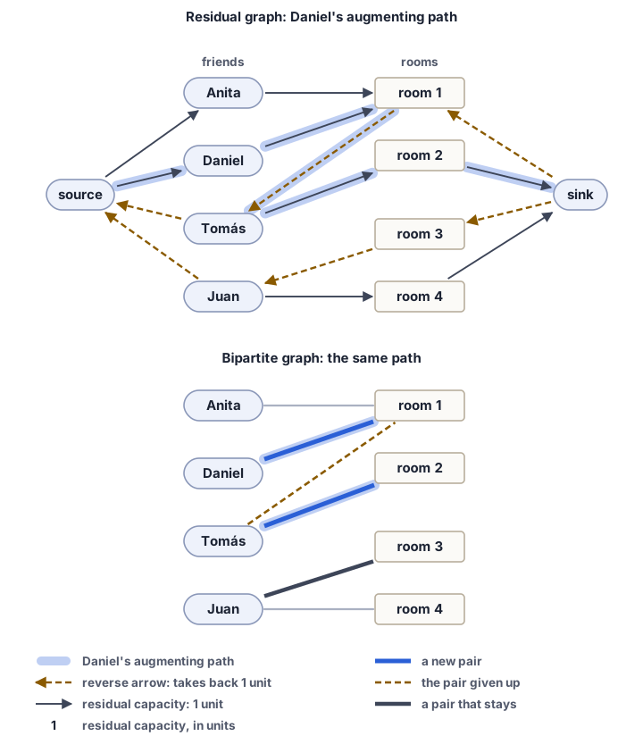
The reduction itself costs little, because it only builds the network and reads back the pairs. Each augmentation adds one pair, and a matching has at most one pair for each person. So a run makes at most one augmentation for each person, and each augmentation costs one search.
With Dinic’s algorithm as the path rule, one search serves a whole round of augmentations. This reduction then becomes the Hopcroft–Karp algorithm [3]. It is the method to use for the largest matching in a bipartite graph when the pairs have no costs. Its work is \(O(m\sqrt{n})\) for \(n\) vertices and \(m\) links.
The matching network also works at a much larger size. At HackMIT 2015, a hackathon at MIT, 359 hackers from out of town each needed a floor to sleep on, and 234 hosts could each take a few of them [4]. Rules such as a hacker’s pet allergy decided which hacker could stay with which host. A greedy pass gave each hacker the first host who fitted and still had a free bed, and it never moved anyone. It placed 95% of the hackers. That left about 18 hackers without a floor. The pass had stopped at a stuck flow, as Daniel’s plan did.
This model differs from the rooms’ matching network only in the beds. A host has several beds, so each host’s arrow to the sink gets a capacity equal to the host’s number of beds (Figure 7.20). The capacities are still integers, so max flow still puts an integer on every arrow, and each unit is one hacker placed with one host. A host with three beds may take three hackers, so the answer is not a matching. The answer’s guarantee comes from the Max flow design box instead.
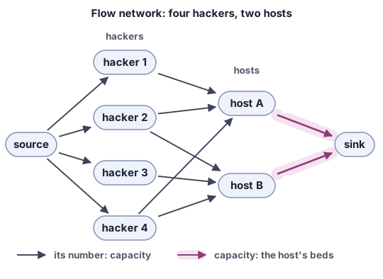
Max flow placed all 359 hackers. When everyone is placed, the count is the proof, since there are only 359 hackers to place.
7.5.2 What stops a larger pairing
Cover certificate; König’s and Hall’s theorems
The run by hand in Section 7.5.1 leaves Anita without a room that she accepts. Anyone can see why the four friends cannot all have one. Anita and Daniel accept only room 1. That makes two people for one room, so one of the two is left out, whatever anyone chooses. Can such a reason always be found, and can the code find it? The maximum matching is a maximum flow on the matching network, with one unit for each matched pair. Its three pairs are a flow of 3 units. So by the max-flow min-cut theorem, the last search’s cut also has a capacity of 3 units (Section 7.3.2).
Reading that cut takes one new term. A vertex and a link are incident when the vertex is one of the link’s ends. A vertex cover, or cover, of a graph is a set of vertices such that every link is incident to at least one of them. A cover can take vertices from both sides. In the flat, the four friends are a cover, and so are the four rooms. Mixing the sides does better: Tomás, Juan and room 1 are a cover of three. Room 1 is incident to the three links into it, Tomás to his link to room 2, and Juan to his two links.
Why does a cover limit every matching? Take a matching and a cover. Remember that a cover is incident to every link, so a set that misses a link is no cover at all. Each pair of the matching is a link, so a member of the cover is incident to it: the pair’s person or its object. Two pairs of a matching never share a person or an object, so different pairs lead to different members of the cover. So, for every matching and every cover,
\[ \text{pairs in the matching} \le \text{members of the cover}. \tag{7.5}\]
So Tomás, Juan and room 1 show that no matching in the flat has more than three pairs. This bound does the job that “no flow exceeds any cut” did in Section 7.3.1.
Take the last search of the run by hand (Figure 7.21). Daniel, Tomás and Juan have rooms, so the source’s arrows to them are full. The search reaches only Anita, then room 1, then Daniel: from room 1 it goes back along the reverse arrow of Daniel’s pair, which is full. Daniel accepts no other room, so the search stops. Its side of the cut holds the source, Anita, Daniel and room 1.
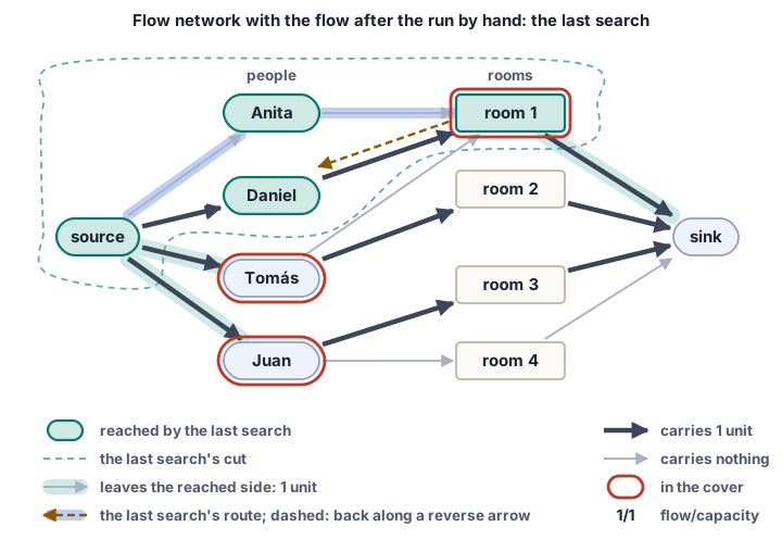
Three arrows leave the reached side, and each one names a member of the cover. The source’s arrow to Tomás names Tomás, the source’s arrow to Juan names Juan, and room 1’s arrow to the sink names room 1. That is the cover of three from before. Only two kinds of arrow can cross like this: one from the source to a person whom the search did not reach, and one to the sink from an object that it did reach. So the cover is the people whom the search does not reach, together with the objects that it does reach, one member for each arrow that crosses, as many as the matching has pairs.
Each arrow that crosses the cut, from the side the search reached to the rest, brings one member of the cover, so the cover has the cut’s size. And every acceptable pair is incident to a member. If the search did not reach the pair’s person, that person is in the cover. If it did, it reached the pair’s object too, and the object is in the cover. An unsaturated pair leads the search on to the object. A saturated pair is the person’s matched pair. Then the person’s arrow from the source is full, so the search can only have come to the person from that object, back along the reverse arrow.
So this matching is a maximum matching, and this cover is a smallest vertex cover. No matching has more pairs than a cover has members, whichever matching and cover you take, and here the two counts are equal. So no matching has more than these three pairs. No cover has fewer than these three members. The cover is the proof. The result is König’s theorem. In a bipartite graph, a maximum matching and a smallest vertex cover have the same size. Dénes König published it in 1931. It is the max-flow min-cut theorem, translated to the matching network. There an integer flow is a matching, one pair for each unit, and the last search’s cut gives a cover, one member for each arrow that crosses it. So “the largest flow equals the smallest cut” becomes “the largest matching equals the smallest cover”.
A second kind of evidence shows why someone is left out. A blocked group is a group of people who together accept fewer objects than the group has people. It leaves someone out in every matching, since its people can be matched only to objects that they accept. Anita and Daniel, who accept only room 1, are a blocked group. Like the graphs chapter’s stuck set, it is evidence that anyone can check, here by counting the objects that its people accept. The same last search finds such a group by itself. When a maximum matching leaves someone unmatched, the people whom the last search reaches form a blocked group. In Figure 7.21 it reached Anita and Daniel, and room 1, the one room that they accept. So every person can be matched exactly when no blocked group exists. This is Hall’s theorem [1, Sec. 7.5], [2], Exercise 25.1-5, which Philip Hall published in 1935.
Where does the guarantee of the Matching design box (The design 7.2) come from? The matching and the cover are max flow’s flow and cut, read on this network. Max flow’s third invariant keeps the flow on every arrow an integer. So each person and each object carries one unit or none, and the flow is a matching. The blocked group is read from the same last search.
The Matching box’s Promise is something that you can demand from any matching code, including code that an AI wrote. Ask for the cover beside the matching. Check that every acceptable pair is incident to a member of the cover, and that the two counts agree. When someone is left out, ask for the blocked group as well. Count the objects that its people accept, and check that there are fewer of them than people.
No choice of rooms gives both Anita and Daniel a room. In this matching Anita gets no room. In another maximum matching Anita is in room 1, and Daniel gets no room. The matching cannot say which of the two should go without, because max flow sees only amounts. Telling such answers apart takes a cost on every arrow. Costs arrive with the next question, the friends’ vehicles.
7.6 Which car collects whose things?
Minimum-cost flow
Sunday morning. Each friend still has one load at their old flat, and the van must go back at noon. That leaves time for one trip each for the van and the friends’ car. The van holds three loads, and the car holds one, so the car collects one load, and the van collects the other three.
Which load goes in the car? Each collection takes effort, and the effort depends on the vehicle and the flat. Daniel lives in a narrow lane, where the van must stop at the corner, but the car reaches his door. Anita’s street is narrow too, but the walk from the corner is shorter. Juan’s desk and Tomás’s bookcase fit in the van, but the car takes them only in pieces. The friends score each collection in points of effort (Table 7.3), and they want the least effort in total.
| van | car | |
|---|---|---|
| Anita | 3 | 2 |
| Daniel | 10 | 5 |
| Juan | 1 | 100 |
| Tomás | 1 | 100 |
Whose load should the car collect, and how would you show that no plan costs less?
Two minutes. You’re done when you have a plan, its cost and a reason.
Now turn the story into a flow network. The effort of one collection becomes the cost of an arrow, as in chapter 6, but now the cost is paid for every unit sent. An arrow of cost 3 that carries two units costs 6.
The source has an arrow of capacity 1 to each old flat, because each flat has one load. Each flat has an arrow of capacity 1 to the van and one to the car. The cost of each such arrow is the effort of that vehicle collecting that flat’s load. The new flat is the sink. The van leads to it with capacity 3, and the car leads to it with capacity 1. The other arrows cost nothing (Figure 7.22). A plan is a flow.
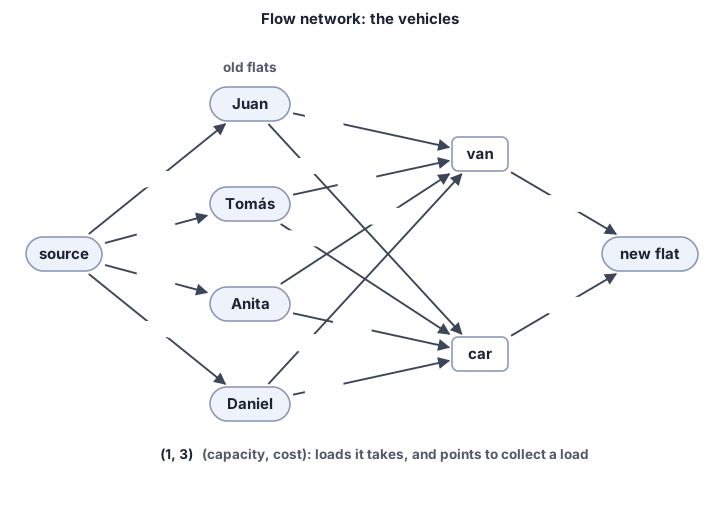
A flow’s cost adds up each arrow’s cost times its flow. The requested amount is given in advance, here four loads, while max flow asked for the largest amount. A cheapest flow has the least cost among all flows of that amount, and textbooks call the problem minimum-cost flow. So you state the network, the costs and the amount, and you ask for a cheapest flow with proof that no flow costs less.
The car takes one load, so only four plans exist, and listing them settles this case. With many loads and vehicles, the plans are far too many to list.
The natural plan picks pairs of a load and a vehicle one at a time. Each time, it takes the cheapest pair that is still possible, and it never undoes a choice. This is cheapest first. Each pair is a path from the source to the sink, so each unit takes chapter 6’s cheapest path among those whose arrows are all unsaturated. Cheapest first rests on a belief that each of its choices stays in the cheapest plan.
Run it. Juan and Tomás go in the van at 1 point each, and Anita goes in the car at 2 points. The car is then full, so Daniel goes in the van at 10 points, for a total of 1 + 1 + 2 + 10 = 14 points. Daniel in the car and the others in the van cost 5 + 3 + 1 + 1 = 10 points. Juan or Tomás in the car costs over 100 points. So 10 points is the cheapest plan (Figure 7.23).
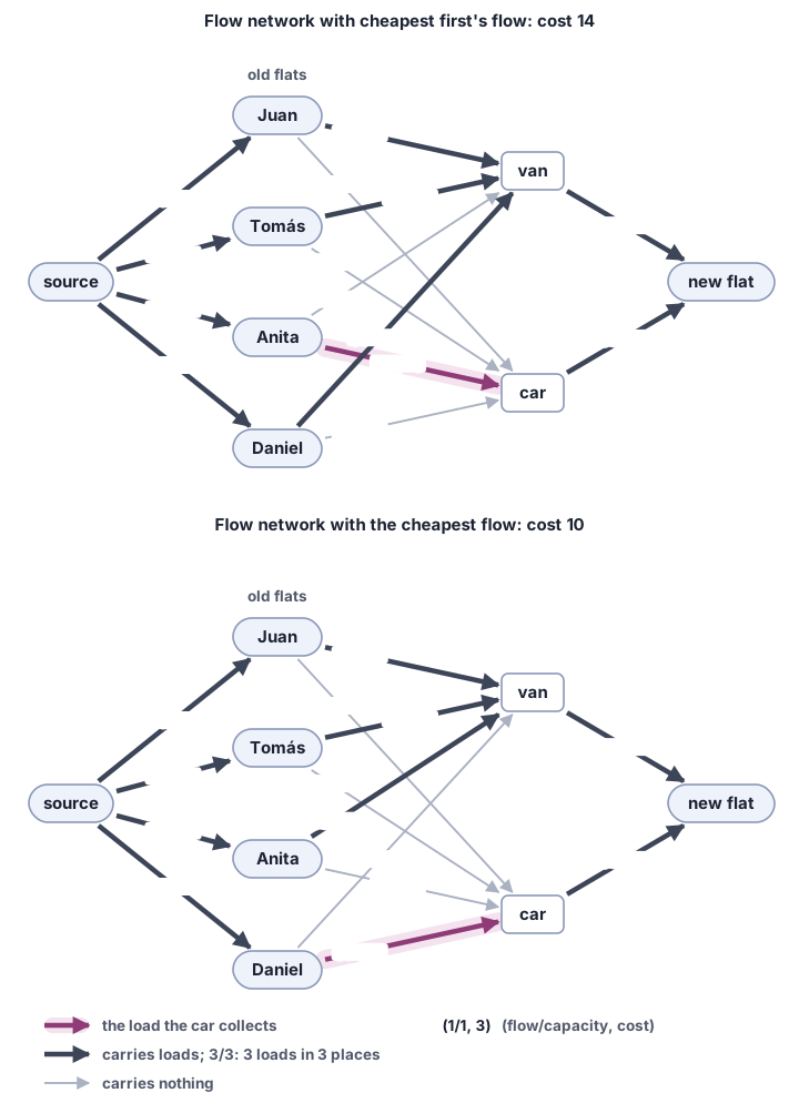
Why does cheapest first pay 4 points too much? The car saves Anita only 1 point against the van, but it would save Daniel 5 points. The car’s one place should go to the biggest saving. Cheapest first looks at one pair at a time, so it never compares two savings.
So the belief is false: one case refutes a rule that is meant for every case. The car has one place, so an early cheap pair can take it from a later load. Anita’s ride in the car must therefore be taken back. In Section 7.2.1, reverse arrows took back flow, and only the amount counted there. What happens to the cost when a load is taken back?
The Min-cost flow design box states the goal, and the idea that the next two sections work out.
7.6.1 Taking a load back refunds its cost
Can the flow of 14 points be repaired without starting over, and how can anyone tell that a flow is the cheapest? That needs a cheaper move that keeps the amount, and a test that no such move is left.
Max flow’s test does not help. No augmenting path is left, because every arrow out of the source is full, yet the flow costs 14 points. That test asks only whether more can be sent, and its residual graph has no costs.
So give every arrow of the residual graph a cost. A forward arrow keeps its cost. A reverse arrow costs minus the cost of the arrow that it reverses, because a unit sent along it takes back an earlier unit, whose cost is no longer paid. A reverse arrow with this negative cost is a refund. With Anita’s load in the car at 2 points, the arrow from the car back to Anita costs −2 points.
Go back to three loads, with Juan and Tomás in the van and Anita in the car. Daniel’s load straight to the van costs 10 points. The augmenting path runs from Daniel to the car (5 points), back to Anita (−2 points) and on to the van (3 points). It costs 5 − 2 + 3 = 6 points (Figure 7.24). The 6 points are a change in the total, not Daniel’s cost. His load costs 5 points, and Anita’s load goes from 2 points to 3.
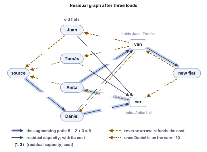
In cheapest first’s finished plan, Daniel’s load is in the van, so the arrow from the van back to Daniel costs −10 points. With this arrow, the path from Daniel through the car and Anita to the van becomes a cycle. A cycle is chapter 5’s path back to its start. Send one unit around it, and the amount stays the same, because every vertex on the cycle takes in one unit and sends out one. The unit changes the total by the cycle’s cost. Here that cost is 5 − 2 + 3 − 10 = −4 points, and the plan of 14 points drops to 10 points. A cycle whose cost is below zero is a negative cycle. In chapter 6 it meant that no cheapest path existed. Here residual capacity limits how many units can go around the cycle, so the cycle is a saving to take.
A flow of the requested amount is the cheapest exactly when its residual graph has no negative cycle. So the test looks for a negative cycle. Ask whoever hands you a flow, a person or an AI, to show that its residual graph has no negative cycle.
Suppose that another flow of the same amount costs less than yours. Compare the two flows arrow by arrow. Where the other flow carries more, the difference runs along your forward arrow. Where it carries less, the difference runs along your reverse arrow. So the difference fits your residual graph. The amounts are equal, so in equals out at every vertex, and the difference splits into cycles, like the boxes going round a loop in Section 7.3.1. The cycles’ costs add up to the other flow’s cost minus yours. That difference is below zero, so at least one cycle is negative.
Refunds have a price. They make some arrows negative, and the next search must handle them.
7.6.2 Heights keep the search safe (and fast!)
Min-cost flow reuses max flow’s loop, the Ford–Fulkerson method of Section 7.4.1: in each round, the path rule adds along an augmenting path of the residual graph. Two things change. The loop stops once the requested amount is sent, and the path rule picks a different path. Edmonds–Karp’s rule takes the path with the fewest arrows, found by breadth-first search. The cheapest path rule takes the path with the least cost, refunds included, so after every round the flow is the cheapest for its new amount. Chapter 6 has two searches for cheapest paths. The Bellman–Ford algorithm accepts negative costs, so it works here as it is, but each round takes \(O(nm)\) time. Dijkstra’s algorithm is much faster, \(O(m \log n)\) a round, but it settles each vertex for good, which is safe only when no arrow is negative (Section 6.3). The refunds bring negative arrows back, so a refund that the search finds later could lower a cost that it has already settled.
Chapter 6’s heights remove this obstacle, so Dijkstra’s algorithm can run (the tilt). Give every vertex \(v\) a height \(h(v)\), and give the arrow from \(u\) to \(v\), with cost \(c(u,v)\), the changed cost
\[ c_h(u,v) = c(u,v) + h(u) - h(v). \tag{7.6}\]
It is A*’s changed cost from Section 6.6.1. Along a path \(P\) from \(s\) to \(t\), the heights cancel except at the two ends:
\[ c_h(P) = c(P) + h(s) - h(t). \tag{7.7}\]
So every path between the same two vertices changes by the same amount, and a path that is cheapest under the costs is also cheapest under the changed costs. The heights are valid when, for every arrow from \(u\) to \(v\) with residual capacity,
\[ c_h(u,v) \ge 0, \tag{7.8}\]
and then Dijkstra’s algorithm is safe. Chapter 6 set its heights once. Here each round opens new reverse arrows, so the heights are updated every round, and valid heights become an invariant that every round must keep.
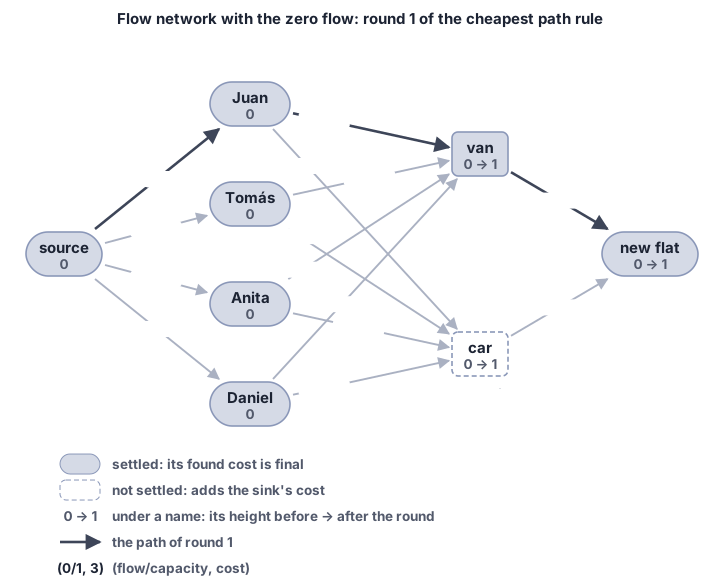
The cheapest path rule puts this together, as one more path rule for the loop. Textbooks call it successive shortest paths [5, Sec. 9.7]. The run starts with no flow and every height zero, which is valid because no cost is negative and no reverse arrow has residual capacity yet. Each round searches best-first on changed costs from the source, sends along the path it found and updates the heights. The search stops once the sink is settled, not when the sink is first reached, because a reached vertex may still get cheaper.
What does a height mean? Dijkstra’s algorithm settles a vertex when its cheapest cost becomes final (chapter 6). This search stops as soon as the sink is settled, so some vertices are settled and the rest are not. After each round, every vertex gets a new height, not only the vertices on the new path. Write \(f(v)\) for the cost that the search found at \(v\), on changed costs. A settled vertex adds its own found cost to its height:
\[ h'(v) = h(v) + f(v). \tag{7.9}\]
A settled vertex’s height is then the real cost of a cheapest path from the source to it, refunds included, in the residual graph that this search used. This follows from equation (7.7): the source keeps height 0, so \(f(v)\) is that real cost minus \(h(v)\). An unsettled vertex’s cost is not final yet, so its height rises by the sink’s found cost \(f(t)\) instead. Its cheapest cost on changed costs is \(f(t)\) or more, because the search settles vertices cheapest first. After the update, every unsaturated arrow has a changed cost of zero or more, and every arrow on the chosen path has a changed cost of zero.
Take round 1 on the vehicles. Every height is 0, so the changed costs are the costs. The search settles the source and the four friends at 0 points, then the van at 1 point through Juan, and the new flat at 1 point, and it stops. It reached the car at 2 points through Anita but did not settle it. So the friends keep height 0, the van and the new flat get height 1, and the car gets the sink’s cost, 1. The car is not on the path, yet its height changes too. The arrow from Anita to the car now has a changed cost of 2 + 0 − 1 = 1, still at least zero (Figure 7.25).
Here it is in code, from min_cost_flow.py.
cheapest_path, is Dijkstra’s algorithm on changed costs, and it sits beside this loop in the module.
On the vehicles network, the first three rounds take what cheapest first took, and round 4 takes Anita’s load back (Figure 7.26). After round 3, the car’s height is 2 and Anita’s height is 0. So the refund from the car to Anita, at −2 points, has the changed cost −2 + 2 − 0 = 0. The search settles the sink at a changed cost of 0 + 3 + 0 + 1 + 0 = 4 points, and adding back the sink’s height of 2 points gives the real 6 points. The plan ends at 10 points.
Why do the heights stay valid? Every height rises by the cost that the search found for its vertex, capped at the sink’s cost. Along an unsaturated arrow, the capped cost at the arrow’s end is at most the capped cost at its start plus the arrow’s changed cost, so the arrow’s changed cost stays zero or more. On each arrow of the path just used, the capped cost at the end is exactly that sum, so the path’s arrows and their new reverse arrows cost zero. So no changed cost is negative, and the flow is the cheapest.
The heights are also the cheapest flow’s certificate. The check needs no trust in the code that found the flow, and it has two steps:
- The flow is legal. It carries the requested amount, it stays within every capacity, and every vertex but the source and the sink sends on what it receives.
- The heights are valid. On each arrow with capacity above 0, the changed cost \(c(u,v) + h(u) - h(v)\) must be \(\ge 0\) when the arrow carries nothing, \(= 0\) when it carries part of its capacity, and \(\le 0\) when it is full (Table 7.4). Together, the three cases say the same as equation (7.8): every arrow with residual capacity, forward or reverse, has a changed cost of zero or more.
| the arrow carries | its changed cost must be |
|---|---|
| nothing | \(\ge 0\) |
| part of its capacity | \(= 0\) |
| its full capacity | \(\le 0\) |
Each step looks at every arrow once. Valid heights alone prove that the flow is the cheapest for its amount. After every round they are valid, and the flow is the cheapest flow of the amount sent so far. The first step checks that this amount is the requested one.
Write \(D(v)\) for the cost that the search found at \(v\), capped at the sink’s found cost: \(f(v)\) for a settled vertex, \(f(t)\) for every other vertex. The update gives every vertex \(h'(v) = h(v) + D(v)\). A settled vertex has \(f(v) \le f(t)\), and every other vertex costs at least \(f(t)\) on changed costs, or the search would have settled it before the sink. So \(D(v)\) is the cheapest cost of reaching \(v\) on changed costs, capped at \(f(t)\).
Take an arrow from \(u\) to \(v\) with residual capacity, and with changed cost \(g \ge 0\) before the update. Reaching \(u\) and then taking the arrow is one way to reach \(v\), so \(v\)’s cheapest cost is at most \(u\)’s cheapest cost plus \(g\). Capping both at \(f(t)\) keeps this, because \(g \ge 0\), so \(D(v) \le D(u) + g\). The arrow’s new changed cost is
\[ g + D(u) - D(v) \ge 0. \tag{7.10}\]
The argument never needs the search to have tried the arrow. So it also covers the arrows out of the sink, which the search never scans, and the arrows between settled and unsettled vertices. Every vertex on the path just used is settled, and along the path \(D(v) = D(u) + g\), so its arrows end at exactly zero, and so do their new reverse arrows. An arrow that the augmentation saturates leaves the residual graph.
Why does that make the flow the cheapest? Around a cycle the heights cancel, so a cycle costs the same under changed costs as under real ones. No changed cost is negative, so no cycle is negative, and by the negative-cycle test of Section 7.6.1 the flow is the cheapest for its amount.
The run ends with these heights: source 0, Juan 5, Tomás 5, Anita 3, Daniel 0, van 6, car 5, new flat 6. Find the changed costs of three reverse arrows: from the van back to Anita, from the van back to Juan and from the car back to Daniel. Then find the changed cost of the arrow from Daniel to the van. Is any of them negative?
Two minutes. You’re done when you have four changed costs.
The three reverse arrows have changed costs of −3 + 6 − 3 = 0, −1 + 6 − 5 = 0 and −5 + 5 − 0 = 0. The arrow from Daniel to the van has a changed cost of 10 + 0 − 6 = 4. The residual graph has 14 unsaturated arrows. Four of them lead back to the source, and eight join the old flats to the vehicles. The last two lead back from the new flat. All 14 have changed costs of at least zero, and 7 of them are exactly zero. So the plan of 10 points is the cheapest, and nobody has to trust the search. Ask for a cheapest flow with its heights, and check every arrow yourself.
Where does the guarantee of the Min-cost flow design box (The design 7.3) come from? The heights prove the cost, the assumption gives the first heights, and the last search’s cut proves the amount when the flow network cannot carry the request, as in Section 7.3.2.
Each round costs one best-first search. In measurements on pixel grids and on sparse random networks, stopping once the sink is settled gave the same answers in a third to a half of the time that settling every vertex took.
7.6.3 What min-cost flow cannot do
The Min-cost flow design box assumes that no cost is negative. But an arrow can earn instead of costing, for example when someone pays for a trip. Under zero heights its changed cost stays negative, and Dijkstra’s algorithm may settle a vertex too early.
Before the first search, the fix is one run of the Bellman–Ford algorithm from a new vertex with a free arrow to every vertex. The cheapest costs that this run finds become valid first heights, because one more arrow cannot lower a cheapest cost. Chapter 6 found heights the same way, in Johnson’s method (Section 6.12) and in the tilt. After that, the heights update keeps the heights valid, as it did for the refunds.
The loop and its heights stay as they are, and they still prove the answer. The price is one run of \(O(nm)\) time. The fix fails when arrows of the flow network form a negative cycle, because then the cheapest cost of reaching a vertex does not exist, so Bellman–Ford gives no starting heights. A cheapest flow can still exist, since capacities limit how much goes around the cycle, but it needs another method, such as cancelling negative cycles. You can state that every cost is at least zero, and check that before the call. Or you can state that costs may be negative but form no negative cycle, and then the code must make the one Bellman–Ford run first. The library’s code takes the first way and refuses any negative cost.
The second limit is speed. Each round sends at least one unit (the loop’s second promise, Section 7.4.1). So a million units may take a million rounds, whatever the network’s size. The path rule cannot choose paths with fewer arrows to save rounds. It must take a cheapest path, however narrow, or the flow may cost more than it needs to. For max flow any augmenting path was right, so Edmonds–Karp and Dinic could take paths with the fewest arrows, and their rounds depend only on \(n\) and \(m\).
So the cheapest path rule suits small amounts. For large amounts, the frontier map (Section 7.14) lists methods whose rounds do not grow with the amount.
The next problem gives every person exactly one room. It takes one search per person, and its costs are zero or more, so it needs no Bellman–Ford run.
7.7 Splitting the rent so nobody envies
The matching could not say whether Anita or Daniel gets room 1. Costs tell such answers apart, as they did for the vehicles, so the friends settle the rooms by price. The rent is 2,000 euros a month. Who takes which room, and how is the rent split so that nobody would rather have another room and pay that room’s share?
Each friend writes what each room is worth to them in euros a month, their value for the room. Each person’s four values add up to the rent (Table 7.5). Tomás has just started his first job, and he can pay at most 450 euros a month.
| Room 1 (courtyard) | Room 2 (courtyard) | Room 3 | Room 4 | |
|---|---|---|---|---|
| Juan | 550 | 400 | 700 | 350 |
| Anita | 700 | 650 | 400 | 250 |
| Daniel | 900 | 550 | 300 | 250 |
| Tomás | 650 | 700 | 400 | 250 |
Anita and Daniel both value room 1 most, at 700 and 900 euros a month, so they cannot both get their favorite.
Counting pairs no longer helps. With prices, every friend takes any room once it is cheap enough. So every pair is acceptable, and every arrangement has four pairs.
The exact route lists every arrangement with its total value. Four friends have 24 arrangements, and listing them takes a few minutes by hand. Ten friends have 3,628,800 arrangements. Twenty friends have about 2.4 × 10¹⁸ arrangements, more than any computer can list. When another method finds an answer, listing can prove it best only by checking every arrangement.
An assignment gives every person exactly one object, and each object goes to exactly one person.
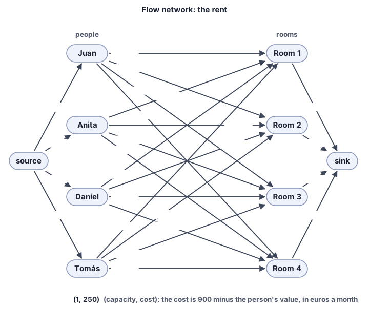
To find one, take the flow network of the quiet rooms and join every person to every object, every arrow with capacity one. This is a reduction, as for matching: a cheapest flow that sends one unit from every person is a cheapest assignment (The design 7.3). The cheapest path rule finds such a flow. Each round sends one whole unit, so each person’s unit goes to a single object. There are as many objects as people, and each object passes on at most one unit, so every object receives one.
The rule finds the least cost, but the friends want the most value. So the arrow from a person to a room costs 900 euros a month minus that person’s value for the room (Figure 7.27). This cost is a number for the method, not a price. The largest value is 900 euros a month, so no cost is negative, as the Min-cost flow design box assumes (The design 7.3). The arrows at the source and the sink cost nothing, so every assignment costs 4 × 900 = 3,600 euros a month minus its total value. The cheapest assignment is the most valued one.
Refunds can take a room back from a friend, as a load was taken back from the car, and heights keep every search safe (Section 7.6.2).
The method finds an assignment and a proof that none costs less, without listing the arrangements. But the method adds values as if a euro meant the same to every friend, and that fails for one friend in the story (Section 7.7.5).
The Assignment design box states the goal, and the idea that the next sections work out.
7.7.1 Labels on both sides
What evidence shows that no assignment costs less than a given one, without listing them all?
The rent’s table has 16 pairs, with costs of up to 650 euros a month. To see the evidence by hand, first take a smaller table: three people, P1, P2 and P3, and three objects, X, Y and Z, with the costs of Table 7.6. Someone gives you the assignment in bold, P1–Z, P2–X, P3–Y, which costs 6 + 2 + 4 = 12. Is 12 the least?
| X | Y | Z | |
|---|---|---|---|
| P1 | 1 | 3 | 6 |
| P2 | 2 | 8 | 9 |
| P3 | 5 | 4 | 9 |
Put a number on each of the three people and on each of the three objects. On every pair, the person’s number and the object’s number must add up to at most the pair’s cost. Make the total of all six numbers as large as you can. Does it reach 12, the cost of P1–Z, P2–X, P3–Y?
Five minutes, by hand. You’re done when you have six numbers that fit every pair and their total, or a reason why they cannot reach 12.
Put a number on every person and every object, and call it a label: \(u_p\) on person \(p\) and \(v_o\) on object \(o\). The labels fit when, on every pair, the two labels add up to at most the pair’s cost. An assignment uses each person and each object once, so each label counts in exactly one of its pairs. The labels fit, so each of those pairs costs at least the sum of its two labels, and the assignment costs at least the labels’ total. Call the pairs that an assignment uses its chosen pairs, and call a pair tight when its two labels add up exactly to its cost. If every chosen pair is tight, the assignment costs exactly the labels’ total, so no assignment costs less. The labels are the assignment’s certificate. The answer to check is the assignment together with one label on every person and every object. The label check has three steps, in one pass over the pairs:
- It is an assignment. Each person and each object is in exactly one chosen pair.
- The labels fit. On every pair, the two labels add up to at most the pair’s cost.
- They meet. Every chosen pair is tight, and the labels add up to the assignment’s cost.
In symbols:
\[ \begin{aligned} u_p + v_o &\le \text{cost}(p, o) && \text{on every pair } (p, o),\\ u_p + v_o &= \text{cost}(p, o) && \text{on every chosen pair } (p, o),\\ \textstyle\sum_p u_p + \sum_o v_o &= \text{cost of the assignment}. \end{aligned} \tag{7.11}\]
| X | Y | Z | label \(u\) | |
|---|---|---|---|---|
| P1 | 1 ≤ 1 | 1 ≤ 3 | 6 ≤ 6 | 1 |
| P2 | 2 ≤ 2 | 2 ≤ 8 | 7 ≤ 9 | 2 |
| P3 | 4 ≤ 5 | 4 ≤ 4 | 9 ≤ 9 | 4 |
| label \(v\) | 0 | 0 | 5 |
On the given assignment, the check passes (Table 7.7). All nine pairs fit, the three chosen pairs are tight, and the labels add up to 1 + 2 + 4 + 0 + 0 + 5 = 12. So no assignment costs less than 12. The labels started from each person’s cheapest cost, 1, 2 and 4, with 0 on every object. They fit, because each person’s label is the cheapest cost in that person’s row, and they total 7. Z’s label could then rise to 5 before any pair in its column stopped fitting, and that raised the total to 12. If your numbers in the Try first box reached 12, they prove the same, even if they differ from these.
The check tests each pair once, and there are nine pairs, which is the number of people squared. For 20 people, the check makes 400 tests, while listing would face about 2.4 × 10¹⁸ assignments (Section 7.7). Checking the labels needs no trust in whoever found the assignment. So you can ask any assignment code for labels with its answer and check them yourself, even when an AI wrote the code.
Labels that fail the check prove nothing either way. Checking labels is easy, but finding labels that are tight on every chosen pair takes a method. The next subsection gives a method that returns them with the assignment. Its labels are the heights of Section 7.6.2, with every person’s height taken with a minus sign.
7.7.2 One person at a time
Section 7.7.1 left one question open. Where do labels that pass the check come from? Place the friends one at a time. How does the next friend get a room that an earlier friend already holds?
The friends enter in the table’s order, with the costs of 900 euros minus each value from Section 7.7. Juan takes room 3, his cheapest, at 200 euros. Anita takes room 1, also at 200 euros. Then Daniel arrives. His cheapest room by far is room 1, at 0 euros, and it is Anita’s.
Should Anita give it up? Against room 2, room 1 saves Daniel 350 euros but saves Anita only 50 euros. So Daniel takes room 1, and Anita moves to room 2. In the flow network, this is one path with a refund (Section 7.6.1): Daniel to room 1 for 0 euros, back from room 1 to Anita for −200 euros, and Anita on to room 2 for 250 euros (Figure 7.28). The total rises by 50 euros, against 350 euros if Daniel went straight to room 2. The path is the alternating path of Section 7.5.1, now the cheapest one.
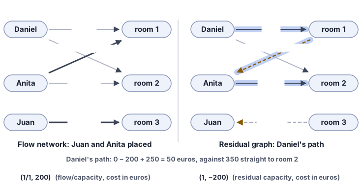
So placing the next person may move earlier people, and one search finds the cheapest way to place that person. Changed costs, heights and the safe search carry over from Section 7.6.2. The run starts with nobody placed and every height zero, which is valid because no cost in the rent’s table is negative. The library’s assignment accepts costs below zero too. Each search starts at the person being placed, and every later arrow leaves a placed person, whose labels already fit. The search starts at the person being placed, as if only that person’s arrow from the source were open. It may end at any free object, whose arrow to the sink still has residual capacity. So no source or sink needs to be drawn. Each search places one more person, so \(n\) people take \(n\) searches.
This is the cheapest path rule with one unit per person, called shortest augmenting path with heights [5, Sec. 12.4]. The search for the person being placed is Dijkstra’s algorithm on changed costs. From a person, the search can go to any object. From an object that someone already has, it can only go back to that person. It stops at the first free object that it settles, and on equal costs it settles a free object first. The heights then move as in the cheapest path rule, with the free object in place of the sink. Then the free object’s cost comes off every height, which leaves every changed cost as it was. That returns every unsettled vertex to its old height, so only the person being placed, the settled objects and their people move. Here it is in code, from assignment.py.
On the rent, take Daniel’s search. After Anita’s step, Anita’s height is −200 and room 1’s height is 0. So the refund from room 1 back to Anita, at −200 euros, has the changed cost −200 + 0 + 200 = 0 euros. The search settles room 1 at 0 euros, then room 2 at 50 euros through Anita’s row, and stops. It finds the same 50 euros by a safe search.
Tomás comes last. His path goes to room 2 for 200 euros, from room 2 back to Anita for −250 euros, and from Anita on to room 4 for 650 euros. That is 600 euros in all, against 650 euros for room 4 directly. So Tomás takes room 2, and Anita moves to room 4. At the end of the run, Juan has room 3, Anita has room 4, Daniel has room 1 and Tomás has room 2. This arrangement costs 1,050 euros, its total value is 2,550 euros, and it is the best of the 24 arrangements (Figure 7.29).
A search settles at most \(n\) objects and scans at most one row of \(n\) costs for each of them, so a search takes about \(n^2\) steps. For 20 people, the \(n\) searches take about 8,000 steps, against about 2.4 × 10¹⁸ arrangements.
Now read the heights as labels. A person’s label is minus the person’s height, and an object’s label is the object’s height. Then “changed cost at least zero” on an arrow from a person to an object reads “the two labels add up to at most the cost”. On the rent, the final labels are 350, 650, 450 and 600 euros on Juan, Anita, Daniel and Tomás, and −450, −400, −150 and 0 euros on rooms 1 to 4. Every pair fits, the chosen pairs are tight, and the labels add up to 1,050 euros, the assignment’s cost. The next subsection reads the room labels.
Why do the labels pass the check? The heights stay valid, so the labels fit every pair. A chosen person can be reached only from their own object, along a refund whose changed cost is zero. So the person’s height and the object’s height move by the same amount, the two labels’ sum stays the same, and every chosen pair stays tight after every search. The labels’ total is a bound that no assignment can go below, and this assignment’s cost meets it, so no assignment costs less. The assignment’s cost bounds the least possible cost from above, and the labels’ total bounds it from below. The assignment and its labels form a primal-dual⬢ pair, an answer and a bound from the other side. The flow and its cut formed such an equal pair too (Section 7.3.2). The matching and its cover formed a third equal pair (Section 7.5.2).
Where does the guarantee of the Assignment design box (The design 7.4) come from? The labels are the cheapest flow’s heights, read on both sides. So the heights’ certificate in the Min-cost flow design box becomes the label check of Section 7.7.1.
7.7.3 Prices nobody envies
The method gave each friend a room (Section 7.7.2). Daniel takes room 1, Tomás takes room 2, Juan takes room 3, and Anita takes room 4. A room’s price is its share of the monthly rent. The friend who takes the room pays that price. The four prices add up to the rent of 2,000 euros. A friend compares rooms by value minus price, which is what they gain from a room at its price. Their favorite after price is a room where they gain the most. The prices are envy-free when no friend gains more from another room than from their own. So which prices leave no friend wanting another friend’s room?
The obvious split is the equal one, 500 euros a room, and it fails. Anita values her room 4 at 250 euros, so she gains 250 − 500 = −250 euros there. In Daniel’s room 1, worth 700 euros to her, she would gain 700 − 500 = 200 euros. Anita envies Daniel. When every room costs the same, each friend still ranks the rooms by value, so the prices must differ.
The labels say how the prices differ. An object’s price is one constant minus its label, and the constant is chosen so that the prices add up to the total to be shared. Then every person’s object is their favorite after price. The method left the labels −450, −400, −150 and 0 euros on rooms 1 to 4 (Section 7.7.2). With the constant 250 euros, room 1’s price is 250 − (−450) = 700 euros, and the four prices are 700, 650, 400 and 250 euros. So the higher the label, the lower the price. The constant changes nothing that a friend compares, because it moves every value minus price by the same amount. So envy leaves the constant open, and the rent fixes it at 250 euros.
Why does this work? Write the label check of Section 7.7.1 in values instead of costs. With \(K\) for the constant, person \(p\) gains value minus price, \((900 - \text{cost}(p, o)) - (K - v_o)\), from object \(o\). Labels that fit make this at most \(900 - K - u_p\), so each person’s label sets the most that the person can gain from any room. A person and their own object form a chosen pair, and every chosen pair is tight. So on their own object, the person gains exactly \(900 - K - u_p\), and no object gives them more. Labels that pass the check therefore always give prices that nobody envies.
In Table 7.8, each friend compares their own room with the three others, so you run 12 comparisons. Juan, for example, gains 300 euros in room 3 and at most 100 euros in any other room. Nobody gains more from another room than from their own.
| Room 1 (price 700 euros) | Room 2 (price 650 euros) | Room 3 (price 400 euros) | Room 4 (price 250 euros) | |
|---|---|---|---|---|
| Juan | −150 | −250 | 300 | 100 |
| Anita | 0 | 0 | 0 | 0 |
| Daniel | 200 | −100 | −100 | 0 |
| Tomás | −50 | 50 | 0 | 0 |
Anita’s row is the edge case. Her value minus price is 0 in every room, so she likes all four rooms exactly as much. A tie is not envy, because no room gives her more than room 4 does. But she gains nothing either, and she is a light sleeper in a street room.
So the split is envy-free, but many other splits are too. Room 1 could cost anything from 637.5 to 850 euros, with the other three prices moved to match, and nobody would envy anyone. The method returns the split in which Anita gains nothing. To pick another split, say one in which every friend gains something, the friends must say what makes a split better. That is a different goal, and the method does not set it.
The check needs only the values table and the four prices with their rooms. It needs neither the method nor trust in whoever ran it, so the prices are the split’s certificate. For n friends the check is n × (n − 1) comparisons. So when someone else splits the rent, or an AI does, ask for the prices with the rooms and run the comparisons.
7.7.4 Where it runs
Two kinds of systems in daily use pair things one to one, many times a second. In both, every pair has a cost, and the pairs together should cost least.
The first is an object detector of the DETR (detection transformer) family, a program that draws a box around each object in a picture. It guesses a fixed number of boxes for every picture, often 100 to 300 boxes, while the picture holds only a handful of real objects. On every training step, it pairs its boxes with the real objects. The cost of a pair says how badly the box fits the object, in class and in place. The boxes are the friends, and the objects are the rooms. The pairing decides which box learns from which object (Figure 7.30).
The second is a tracker, which follows people through a video. On every frame, it pairs the new detections with the people that it follows. The cost of a pair is how far a detection lies from where that person was expected. The tracker’s designer also writes down a largest cost that a pair may have, and a detection whose cost is above that limit for every person starts a new person. That largest cost is a requirement written into the table, and the method stays the same.
The obvious way is cheapest first, the rule that failed the vehicles in Section 7.6. It takes the cheapest pair left and never undoes a choice. But an early cheap pair can take an object that someone else needed more. On the 3×3 table of Section 7.7.1, cheapest first takes P1–X for 1, then P3–Y for 4, then P2–Z for 9. That makes 14, and the labels proved that the cheapest assignment costs 12.
These systems run the method of Section 7.7.2 (the Assignment design box). DETR-family detectors call SciPy’s linear_sum_assignment, and trackers call LAPJV or SciPy. Libraries and papers call this family the Hungarian method, the name that Kuhn gave it in 1955. The chapter’s method is its modern form, one cheapest path per person.
A detector has more boxes than objects. The assignment still applies once the short side is filled with stand-in objects that all cost the same. A box that gets a stand-in learns “no object”. The stand-ins do not change which real pairs are best, because every assignment of the filled table pays the same total for its stand-ins.
These routines return the pairs alone. The chapter’s method also returns the labels, so you can ask for them and run the label check on every result.
On three tables of 100, 1,000 and 3,000 people generated for this book, where each person may take only 8 objects, cheapest first left about 9 people in 100 without any object, although an assignment that places everyone exists. The chapter’s method needs longer code than cheapest first, and in return it places everyone whenever that is possible.
7.7.5 What the rent split cannot do
This subsection names four limits of the chapter’s methods, from max flow to the assignment. The first limit is about amounts. Max flow and matching cannot rank two flows of the same amount or two largest matchings. The rooms have four largest matchings of three pairs, all correct for the Matching design box. Two path rules can stop at different maximum flows, both correct for the Max flow design box.
An arrow carries only a capacity, and an acceptable pair is a yes or a no. Chapter 6 weighed each arrow by its cost, the right measure for one path. Max flow asks how much fits through many paths, and only capacities decide that. Costs rank the answers, for the vehicles and for the rent.
The second limit is about integers. With capacities that are not integers, an arbitrary path rule may augment forever, toward an amount below the maximum. In one small flow network a capacity is (√5 − 1)/2, about 0.618, and a bad order of augmenting paths never finishes [6].
The second promise of Section 7.4.1 asked for at least one whole unit per round. With fractional capacities, an addition can be smaller than one unit. For example, the running total of ½ + ¼ + ⅛ + … grows at every step and never reaches 1. The additions can shrink the same way toward a finite total, so the flow rises at every step yet never reaches the maximum. Fractions alone are harmless, because in a small enough unit they are integers, and the count of augmentations holds again (Section 7.4). Only capacities with no common unit, such as (√5 − 1)/2 beside integers, can make a run endless.
So an arbitrary path rule needs integers in a common unit. The chapter’s Edmonds–Karp and capacity scaling need them too, because their searches follow only arrows with at least one unit of residual capacity. With capacities that have no common unit, these two may stop below the maximum. Dinic finishes on any capacities. An Edmonds–Karp whose search follows every unsaturated arrow finishes on any capacities too. The bounds of Dinic and of this Edmonds–Karp count arrows and vertices, never units. For Edmonds–Karp, the count was how often each arrow can fill while the distance from the source never shrinks (Section 7.4.2). For Dinic, the count was the rounds, by the sink’s layer (Section 7.4.3).
The third limit is about two sides. The matching reduction pairs people with objects. When any two people may pair, there are no two sides. That is general matching, where links may join any two vertices and each vertex is still in at most one pair.
The matching network sends every unit through one person and one object, so every vertex other than the source and the sink has one role, person or object. A person who may pair with another person needs both roles, and copying each person onto both sides does not help. On three people who all accept each other, the reduction with copies returns three pairs, first with second, second with third and third with first. Each person sits in two of them, so they form a cycle, not a matching.
The certificate also stops meeting the answer. Any pair leaves the third person alone, so the largest matching has one pair. One person is incident to only two of the three links, so a vertex cover needs two people. So König’s equality from Section 7.5.2 fails here (Figure 7.31).
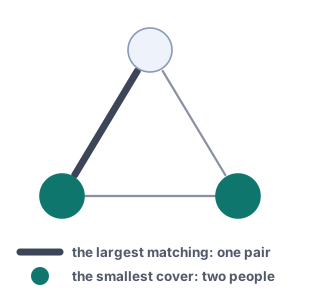
General matching needs its own method, which this book does not teach. Chapter 9 uses such a method through its contract, to pair up a tree’s vertices that have an odd number of links at the least total cost. When you hand a matching problem over, say whether it has two sides.
Last, at the label prices, all 12 envy comparisons pass and the total value is the largest. Yet Tomás gets room 2 at 650 euros a month, 200 euros a month over what he can pay. Every set of prices that nobody envies puts room 2 at 550 euros a month or more (Figure 7.32).
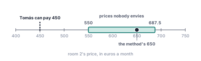
The method made the total value as large as possible, and that total is its objective, the one number that a method makes best. The method takes in only the values. Tomás’s 700 euros a month for room 2 says how much he likes it, not what he can pay, so the largest total puts him there. He could not have kept all four values under 450 euros a month either, since they must add up to the rent of 2,000 euros a month. Prices that nobody envies cannot move him, because such prices exist only for a best assignment. Take any other assignment. Under the prices, each friend likes their own room after price at least as much as their room in the other assignment. Add these comparisons over all friends. The prices cancel, because both assignments pay the whole rent. So that assignment’s total value is no larger. Economists call an assignment with prices that nobody envies a competitive equilibrium. They call this result the first welfare theorem. For assignments, Lloyd Shapley and Martin Shubik proved it in 1971 [7, Sec. 3.2], p. 119. Here only one assignment is best, so Tomás stays in room 2.
So the labels prove that the assignment is best for the objective as written. They do not prove that its people meant that objective. Choosing and writing it is their job, not a certificate’s. “Optimal, so right” does not follow, because an assignment that is not the best fails the label check, but the best assignment for a wrong objective passes it. As the preface put it, “An objective can be optimized perfectly while omitting something we cared about.”
The friends can add the budget as a requirement, or choose another objective. For each choice, a tool or an AI can find an assignment, and the friends check its certificate before they choose. Here the budget conflicts with prices that nobody envies, so one must go.
Every main answer of this chapter came with evidence that anyone can check, and the next section says what that evidence shares.
7.8 What is this all about?
The building’s flow of two boxes a minute came with a cut of the same capacity around the vertices that the last search reached (Section 7.3.2). On the matching network, the same kind of cut became a cover (Section 7.5.2). The vehicles’ cheapest flow came with heights (Section 7.6.2), and the rent assignment came with labels (Section 7.7.2). What did each attach numbers to, what did those numbers bound, and why does checking them prove the answer best?
Chapter 1 promised answers that carry their own evidence.
Each answer comes with markings on the vertices, and each marking is a number. The cut puts 0 on the source’s side and 1 on the sink’s side. The cover puts 1 on its members and 0 elsewhere, and the labels are numbers already. For the largest flow, the matching and the assignment, these markings let you calculate a bound that no possible answer can beat, and the bound meets the answer. The cheapest flow’s heights work another way. They show that no negative cycle is left, and the cheapest flow’s bound waits for chapter 8. The last column of Table 7.9 names the numbers that meet.
Why is meeting enough? The bound holds for every possible answer, just as no flow exceeds any cut (Section 7.3.1). So an answer that meets it cannot be beaten.
So the check has three parts. First, the answer must be legal. A flow, with costs or without, stays within every capacity, and every vertex but the source and the sink sends on what it receives. A matching uses only acceptable pairs and no person or object twice. An assignment uses each person and object exactly once. Second, the markings must be valid. The cut marks the source 0 and the sink 1, and the cover, the heights and the labels satisfy the third column’s check. Third, where the last column names two numbers, they must be equal.
| answer | markings on the vertices | check on every link or pair | two numbers that must be equal |
|---|---|---|---|
| largest flow | the cut’s sides, 0 and 1 | none | the flow amount and the capacity of the arrows from 0 to 1 |
| maximum matching | the cut on the matching network, read as a cover | every link is incident to a member of the cover | the number of pairs and the number of cover members |
| cheapest flow | the heights | every unsaturated arrow has a changed cost of at least zero | a bound exists; chapter 8 derives it |
| assignment | the labels | on every pair, the two labels add up to at most the pair’s cost | the assignment’s cost and the total of the labels |
In 1955, Theodore Harris and Frank Ross studied where bombing would cut a railway network. They found a flow beside a cut of the same capacity [8, pp. 442–443]. Their study reads as a contest: one party sends, and the other blocks. The answer is the sending party’s move, and the markings are the blocking party’s move. The cover and the labels block like the cut, and chapter 8 shows that the heights block too.
Building an answer together with the bound that proves it is the primal-dual primitive of Section 7.7.2. Chapter 8 builds this pairing of sending and blocking into linear programming duality, and it renames heights, labels and changed costs.
The gain is trust that does not depend on the solver. The check is small enough to write and verify apart from the method that found the answer. Each part of the check reads the network once. So the check’s time grows with the network’s size, while the run took many searches. The markings also support decisions. The minimum cuts showed that the furniture lift pays off, and the labels became prices that nobody envies.
A certifying algorithm pairs a fast solver, which nobody needs to trust, with a small checker that is trusted [9]. So ask any tool or AI for the certificate beside its answer, and run the check yourself.
A passing check proves an answer best only for the objective as written. The rent assignment passed every check, yet Tomás cannot pay for his room (Section 7.7.5).
A second limit is that not every method returns a certificate. The cut without a source is found by random contraction, and repeats raise confidence but never prove the cut smallest.
Many problems that never mention a flow become a cut or a flow on the right network, and the certificate comes with the answer. The hard part is building that network. For example, which products should a firm keep? How many routes share no arrow? That is chapter 5’s question of what survives a failure. Can a team still win its league? The self-check problems of Section 7.13 build these networks.
The next section gives you a changed setting, and you decide without AI which answers and certificates still hold.
7.9 ✎ When assumptions change practice
So far, every answer has come with a certificate, and both were computed for one flow network. After a change, check both against the new network. If the answer still keeps the lines of its design box and the certificate still passes its check, nothing runs again. If not, the line that broke says what must run again.
At noon, Juan’s flow moves two boxes a minute into the flat. One box a minute takes the front door and the lift, and the other takes the courtyard gate and the back stairs. Then the lift breaks down, so its capacity is now 0 boxes a minute. Which line of the Max flow design box (The design 7.1) does Juan’s flow break? Is its amount now wrong? Does the old cut through the front door and the courtyard gate still prove anything? What would you run again, and from which flow? Find the new largest amount and the cut that proves it.
A ride service wants to match as many riders as possible to nearby drivers, each driver taking at most one rider. Model this as a matching network: what are the vertices, arrows and capacities? Then a rule says that some riders must not be matched to some drivers. Where does that rule go, and does the cover of the Matching design box (The design 7.2) still prove that your matching is the largest? If the rule comes after the matching, what has to run again?
In the rent table (Table 7.5), each cost is 900 euros a month minus a value. Suppose the landlord pays Juan 400 euros a month to take room 1. His value then rises from 550 to 950 euros a month, so this pair costs \(900 - 950 = -50\) euros a month. Do the final labels of Section 7.7.2 still pass the label check? Does any line of the Assignment design box (The design 7.4) break? Which step of that section no longer reads as written? How would you change the costs so that it does, without changing which assignment is cheapest?
7.10 ◆ What these are actually made of big picture
This chapter put four methods in design boxes: max flow, matching, cheapest flow and assignment. Open them up, and each one is a few primitives put together.
Each part is a primitive of the book’s catalog, named beside the place where it first worked:
- residual state: Section 7.2.1;
- augmentation: Section 7.2.2;
- cut certifies flow: Section 7.3.2;
- reduction: chapter 5, then Section 7.5.1;
- keep an invariant: chapter 1;
- best-first search: chapter 4;
- primal-dual: Section 7.7.2.
Seven primitives make all four methods. Figure 7.33 writes each method as a row of chips.
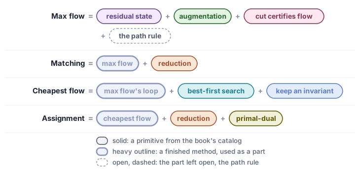
Max flow = residual state + augmentation + cut certifies flow, with the path rule left open. Residual state: every unit sent leaves a reverse arrow, so a later path can take that unit back. Augmentation: add along an augmenting path until none is left. Cut certifies flow: the cut around the vertices that the last search reaches has a capacity equal to the flow amount.
Matching = max flow + reduction. Reduction: the matching network gives one unit of capacity from the source to every person, along every acceptable pair, and from every object to the sink. The flow is an integer flow, so a maximum flow is a maximum matching. The same last search gives the vertex cover.
Cheapest flow = max flow’s loop + best-first search + keep an invariant. Best-first search: the path rule takes the cheapest augmenting path, which Dijkstra’s algorithm finds on the changed costs. Keep an invariant: valid heights keep every unsaturated arrow at a changed cost of at least zero, so Dijkstra’s search stays safe.
Assignment = cheapest flow + reduction + primal-dual. The cheapest flow runs on the matching network with costs, one person at a time. Primal-dual: the heights become the labels, and the labels add up to a bound that meets the assignment’s cost.
So no later method needed a new idea of a loop. Each repeats max flow’s pattern of repairs, though its code runs its own loop, and adds only what its own promise needs, such as the heights that prove a flow the cheapest.
Outside the main text, two methods do without the loop. Push-relabel still returns a maximum flow and its cut (appendix). Repeated many times, Karger’s algorithm is likely to find the fewest links that split an undirected graph, but it returns no certificate (appendix).
The methods differ in three choices. Each method makes these choices in its own way.
- The path rule. Ford–Fulkerson by hand takes any augmenting path. Edmonds–Karp takes the path with the fewest arrows. Dinic’s algorithm takes a round through the layers. Capacity scaling takes only paths with at least a threshold of residual capacity. Cheapest flow and assignment take the cheapest path on the changed costs.
- The network. Max flow runs on the given network. Matching runs on the matching network, which a reduction builds. Cheapest flow runs on a network with a cost on every arrow. Assignment runs on the matching network with costs.
- The stop. Max flow and matching stop when no augmenting path is left. Cheapest flow stops at the requested amount. Assignment stops when every person has an object.
Beside each part that this chapter uses, Figure 7.34 shows five swaps that keep the promise and one that breaks it.
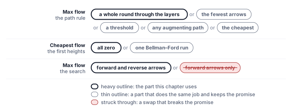
In the first row, this chapter’s path rule is Dinic’s, the library’s default. Each of the four swaps keeps the three promises of Section 7.4.1, so the loop’s one proof covers it.
In the second row, one Bellman–Ford run can replace the zero first heights when some cost is negative, as in Section 7.6.3.
In the third row, the struck-through search takes only forward arrows, not every residual arrow, so it can stop below the maximum flow, as Daniel’s flow did in Section 7.2. It reports that no path is left while one through a reverse arrow remains. So residual state is the one part that no path rule may drop.
7.10.1 Choosing one, under pressure
Suppose that a problem asks you to send or share out something scarce. Which method answers it, what certificate comes back, and what must hold for the answer to be right? Each row of Table 7.10 is a short contract in chapter 1’s sense.
Two assumptions can fail. The first is what a right answer needs. When it fails, the input is refused, or the method may never finish. The second is what makes the method the right pick. When it fails, the answer is right and passes its check, but it answers another question.
| The question | The method | The certificate beside it | What it relies on, and what happens when that fails |
|---|---|---|---|
| the most that can be sent from one source to one sink | max flow, with Dinic’s rule unless another path rule is named | a cut whose capacity equals the flow amount | Integer capacities, unless the path rule is Dinic. Without them, the chapter’s Edmonds–Karp and capacity scaling may stop below the maximum, and another path rule may never finish. Max flow also sees only amounts, so with costs, use the cheapest flow. |
| as many pairs as possible, each person with an object that the person accepts | matching, by max flow on the matching network | a vertex cover with as many members as the matching has pairs | Two sides and no costs. People matched among themselves need general matching (chapter 9). With costs on pairs, use the assignment when every person takes exactly one object, and use the cheapest flow otherwise. |
| the cheapest way to send a requested amount from one source to one sink | cheapest flow, one cheapest path at a time | heights: every unsaturated arrow has a changed cost of at least zero | No negative costs, unless valid heights are found first. The work grows with the amount, so large amounts need another method (Section 7.6.3). |
| every person gets one object, at the least total cost | the assignment, one person at a time | a label on every person and every object: on every pair, the two labels add up to at most the pair’s cost, and on every chosen pair they add up to exactly that cost | As many objects as people. A table of another shape is refused. The objective as written must also be the objective that you meant. When the two differ, the labels still pass. |
Name the question first, because it picks the row. Max flow leaves a second pick, the path rule, and so does matching, which runs max flow. That pick follows the workload (Figure 7.16), because on integer capacities a wrong pick costs time, never correctness. Dinic is the default. Edmonds–Karp fits when the code must stay smallest. Capacity scaling fits long flow networks whose capacities span a wide range. Push-relabel fits large general networks (appendix).
Only the second kind of failure, a right answer to another question, gets past the certificate (Section 7.7.5).
7.10.2 What each one costs
What does each method cost? How does its work grow with the flow network, and how long does one call take? A network has \(n\) vertices and \(m\) arrows. For matching, \(n\) counts the people and the objects, and \(m\) counts the acceptable pairs. For the assignment, \(n\) is the number of people, and the table has \(n\) rows of \(n\) costs.
Each row of Table 7.11 gives two measures. The formula, written with \(O\), gives an upper bound on the method’s work. The measured call is how long one call of the library takes on one network.
| Method | Formula | Measured call |
|---|---|---|
| Edmonds–Karp | \(O(nm^2)\) | 16.9 s, on 65,538 vertices and 328,990 arrows |
| Dinic’s algorithm, the library’s default | \(O(n^2 m)\) | 92 ms, on the same network |
| matching | \(O(n + m)\) to build the network, then \(O(nm)\), with at most one augmentation per person; \(O(m\sqrt{n})\) with Dinic’s rule, the Hopcroft–Karp bound | 116 ms, on 65,536 people, 65,536 objects and 524,288 acceptable pairs |
| cheapest flow | \(O(F (n + m) \log n)\) for \(F\) units, with one best-first search per step | 3.7 s, sending 3,841 units on 16,386 vertices and 65,280 arrows |
| assignment | \(O(n^3)\) on a full table, with one search of \(O(n^2)\) per person | 22 ms, on 1,000 people and 1,000,000 costs |
Big \(O\) is asymptotic. It says how the work grows as the network grows, and leaves out constant factors and small networks.
The formula holds on every network of a given size and compares methods before anything runs. The formula’s gain is prediction. Give the assignment twice as many people, and the bound in its formula becomes about eight times as large, because \(2^3 = 8\). A measured time holds only for the network that was timed, so time the method on your own networks.
7.10.3 The same ideas, over and over
The ideas behind the chapter’s methods also run outside it. Panorama stitching, object detection, reviewer assignment and chip design use them, and so do the next two chapters. Each row of Table 7.12 puts one of five ideas beside the systems that run it.
| Idea | Where else it runs |
|---|---|
| residual state | undoing a move, in chapter 9’s local search on hard problems, where improving moves can stop short of the best answer |
| augmentation | the assignment that DETR-family detectors solve on every training step (Section 7.7.4); the simplex method of chapter 8 |
| cut certifies flow | the seam that OpenCV’s panorama stitcher draws between two photos, which is a minimum cut; chapter 8, where the max-flow min-cut theorem becomes one case of a theorem about linear programs |
| reduction | reviewers to papers, each reviewer with a quota, in OpenReview’s matcher; clock-tree sink clustering in the OpenROAD chip-design flow; each one solved as a cheapest flow |
| heights | push-relabel (Section 7.15); the prices on constraints in chapter 8 |
A row names an idea, not this chapter’s code. OpenCV chooses its augmenting paths by Boykov and Kolmogorov’s rule, and OpenROAD solves its cheapest flows by network simplex. So OpenCV swapped the path rule, and OpenROAD swapped the whole solver.
7.11 ◆ Where that leaves the flat big picture
Moving day asked four questions, and one difficulty stood behind all of them. By Sunday noon, each answer has its evidence, and only Tomás’s room is wrong. One loop answered all four questions with two moves, and a third move is the job of the people who state the problem.
The first move is repair. The corridor’s box was canceled on paper, Tomás gave up room 1 for Daniel, and Anita’s load came back from the car. Every unit sent leaves a reverse arrow, so a later repair path can undo it without starting over.
The second move is evidence. Only two boxes a minute cross one line through the building. Anita and Daniel accept only room 1. The heights show that no plan for the vehicles costs less, and nobody envies anyone at the prices. Each fact rests on vertex markings that anyone can check without trusting the solver.
The third move is a judgment, and someone must take responsibility for it: is the goal that was written the goal that was meant? The assignment is best for its objective, and its split is envy-free, yet Tomás cannot afford his room.
The first two moves come from one loop of repairs. Its last search gives the line or the cover. Every search of the assignment keeps the labels fitting every pair and tight on the chosen pairs. The third move lies outside the loop, since the evidence proves the answer best only for the objective that was written. These three moves answer the difficulty raised in Section 7.1: how can anyone tell whether a better plan exists?
Design moves that can repair an earlier choice, return evidence that the result is best, and check that “best” is the goal you wrote.
7.12 ✎ Hands-on projects practice
The projects come first. In each one you build something, measure something, or explain something to another person. A project has no single right answer, so you judge your work by the checks that it asks you to build. After the projects come the self-check problems, each with an answer that you can check. When a project needs code, let an AI write it. But three things are still your job when the AI helps, in this order. You say what the code must do. You build the check that shows the code does it. And you judge what comes back.
Project 1 · checking · medium · ~1.5 hours
An allocator that may leave people out. You have people and objects, and each object has a number of seats. Each person has a cost for each object, a number between 0 and a largest cost \(C\). Some people may be left out, because the seats run short or a person’s seat costs more than the price of leaving that person out. An AI will write the allocator. How will you know that its answer is the cheapest, and that the cheapest is the allocation that you meant?
The assignment of Section 7.7.2 cannot take this problem as it stands. It takes a square table and gives every person exactly one object. Its design box says so: “As many objects as people.” This project reduces the other shapes to that one.
So reduce the problem to the box, with three changes to the table.
- Copy each object once per seat. An object with three seats becomes three copies, and each copy is an ordinary object that takes one person. This is called cloning.
- Add “none”. Add one extra object for each person, called “none”. Its cost is the penalty for none, the price of leaving that person out.
- Pad to a square. Objects now outnumber people, so add stand-in people who cost 0 on every object.
Now the box applies unchanged. Its label check covers the copies and the “none” objects in one pass.
One number is still open, the penalty. The person who states the problem makes this choice (Section 7.7.5), and it decides the objective. A small penalty lets the cheapest plan leave people out. The same penalty \(P\) for everyone, with \(P\) larger than \(nC\), makes the plan serve as many people as possible first. Here \(n\) is the number of people. Why is that enough? Take two plans, where the second serves more people than the first. The second plan leaves out fewer people. So it saves \(P\) or more in penalties. Its assignment costs add up to at most \(nC\), because it assigns at most \(n\) people and each cost is at most \(C\). So when \(P\) is larger than \(nC\), the second plan is cheaper. This bound is enough, but a smaller \(P\) may already serve as many people as possible.
On the next instance, a small penalty and a penalty above \(nC\) give different plans. Take three people and two objects. Object X has two seats, and the first, second and third person cost 1, 2 and 3 on it. Object Y has one seat, and it costs 8 for each of them, so \(C\) is 8. Compute \(nC\) for this instance, and pick an integer \(P\) above it. Run your model once with \(P = 3\) and once with your \(P\). For each run, say what the plan costs and who it leaves out, if anyone. Then say whether both plans pass the label check.
The reduction changed the table, not the method. One model and one label check judge both penalties. But the check proves a plan cheapest only for the objective that you wrote. Finish with one question. The labels pass, so why might you still reject this allocation? Say which mistakes the label check catches, and which mistakes pass it.
\(nC\) is 24, so take \(P\) = 25. With \(P\) = 3, the plan costs 6: the people take X, X and none, so the third person is left out at the penalty 3. With \(P\) = 25, the plan costs 11: the people take X, X and Y, and nobody is left out. Both plans pass the label check on the reduced table. Each is the only cheapest allocation of the real seats. On the reduced table the assignment is unique only up to swapping the copies of one object, the “none” objects or the stand-in people, which changes no allocation.
Project 2 · design · hard · ~3 hours
Choose a path rule for your own flow networks, with an AI. Your problem is to find a path rule with three properties. It keeps the max-flow promise on your networks. It meets a speed requirement that you choose. And no other path rule beats it on both code size and time.
- Write the problem first. Write four lines of a box: goal, promise, cost and assumptions. Leave the idea and the invariants empty. Pick the speed requirement from a menu of three: at most \(n\) rounds, at most \(nm\) added paths, or a bound in \(n\) and \(m\) that you state yourself. Here \(n\) is the number of vertices, and \(m\) is the number of arrows.
- Check the promise where a machine holds it. Compare your promise, line by line, with
Workbench.Contractin the library’sWorkbench/Spec.lean. It is the contract that every candidate owes. A candidate must return a flow and, beside it, a cut whose capacity equals the flow amount. It must reach that flow along augmenting paths, and each path must carry at least one unit. Where your promise says something else, change it, or say why the contract is wrong. - Let an AI write several path rules. Each path rule is a start and a round. The bench,
algodesign.flows.workbenchinworkbench.py, is Python, so the AI writes in Python, and the times it reports are Python’s, on your machine. Run them on the bench beside the library’s Edmonds–Karp, Dinic and capacity scaling. Judge them on networks of your own that you keep from the AI, so that a path rule cannot win by being tuned to the networks that the AI has seen. - Let the bench check every answer. The bench trusts no path rule. It replays every round on its own copy of the residual capacities, so every path must be augmenting when its turn comes. At the end it accepts an answer only when the vertices that it still reaches from the source give a cut whose capacity equals the flow amount. A flow whose amount equals a cut’s capacity is a maximum flow, since no flow exceeds any cut (Section 7.3.2).
- Choose. The bench counts rounds, measures time and code size, and keeps the path rules that no other one beats on both code size and time. They form the Pareto frontier of Section 7.4.4. Pick from it by your own workload.
The bench sees only the networks that you bring, so it checks your stated bound only on those networks. Reading the code is still your job.
Hand in the final box, with a line for each change, saying whether it fixed the code, the box or the design. ★ Prove in Lean that your path rule keeps the promise of Section 7.4.1 and meets your speed requirement. The contract then follows from them.
This run chose at most \(n\) rounds, and its promise was checked line by line against Workbench.Contract.
The AI wrote three path rules. One groups shortest paths by length into rounds, one is Dinic, and one walks down distance labels to the sink. The AI warned that a path rule could meet the round limit by doing all its work in one round.
All three passed the bench on 15 networks and on 20,000 small random ones. The bench rejected the library’s Edmonds–Karp and capacity scaling. Edmonds–Karp needed 144 rounds on a network of 26 vertices. There, 144 arrows of capacity 1 join 12 vertices to 12 others, and the source’s and the sink’s arrows have capacity 12. That network was added before the AI’s path rules came back, because every path rule passed on the first networks.
The time showed what the rounds hid. The grouped rule used 22 rounds over the 15 networks, as Dinic did, but it sent Edmonds–Karp’s paths with one search for each. It took 17.9 milliseconds, nearly as long as the 22.5 milliseconds of Edmonds–Karp. The AI’s Dinic took 3.1 milliseconds with 44 lines of code. The library’s Dinic, which also counts its steps, took 5.3 milliseconds with 50 lines. The label rule tied with the AI’s Dinic on time and had more code. On the two matching networks, the AI’s Dinic took 0.49 milliseconds and the label rule took 0.64 milliseconds. On the grids and the random networks, the label rule needed a fifth to a third less time than the AI’s Dinic. Pick the AI’s Dinic for matching networks. Pick the label rule for grids and random networks.
SciPy’s function for a maximum matching, maximum_bipartite_matching, runs the Hopcroft–Karp algorithm, which is Dinic on the matching network (Section 7.5.1). The function’s depth-first search never marked a vertex whose search had failed. So on a layered graph it searched such a vertex again whenever another path reached the vertex. Every matching it returned was right. A user measured 8.8 seconds on a graph of 94 vertices, and the time doubled with every added layer, until the fix in 2026 [10], [11].
- Before running anything, draw a ladder of three layers. Each layer has two vertices, and both are joined to both vertices of the next layer. No path from the ladder reaches the sink. One vertex outside the ladder is joined to both vertices of its first layer. Suppose the search reaches this vertex and tries the ladder before a short path to the sink. Count how many times it enters a ladder vertex when nothing is marked, and how many times it enters one when each dead end is marked.
- Say which part of Section 7.4.3 forbids this blow-up in Dinic.
- Say why no certificate of this chapter could have caught the bug. On the bench of Project 2, the measured time would have caught it, and the counts of rounds and added paths would not.
Only after you have your own answer, describe the ladder to an AI and ask for the same count. Does it run the steps, or does it recite the bound that the function promised?
7.13 ✎ Self-check problems practice
Everything these problems need is in this chapter. Each Transfer has its answer in a fold, and the exercises’ answers are on a page of their own.
Transfer 1 · middling · ~30 min
Prices for the experts. A large language model can be built from parts called experts, and a router scores each piece of text, called a token, against each expert (Table 7.13).
| Token | A | B | C | D |
|---|---|---|---|---|
| 1 | 6 | 8 | 2 | 3 |
| 2 | 3 | 4 | 5 | 3 |
| 3 | 7 | 5 | 9 | 4 |
| 4 | 3 | 9 | 4 | 1 |
| 5 | 2 | 7 | 4 | 9 |
| 6 | 2 | 8 | 3 | 4 |
| 7 | 8 | 3 | 2 | 9 |
| 8 | 5 | 7 | 1 | 1 |
Each expert must take exactly two tokens. With one price for each expert, a token takes the expert with the largest score minus price. Call that expert the token’s favorite after price. Which routing scores most, and which prices make every token pick its expert in that routing?
If every token goes to its top score, tokens 1, 4, 6 and 8 all go to B, and A gets no token.
Give each expert two seats, as two copies of the expert. The tokens are the people, and the copies are the objects, with the scores as values. Solve the assignment, and set each copy’s price to one constant minus its label.
The assignment gives A {1, 8}, B {4, 6}, C {2, 3} and D {5, 7}, with a score of 60 points. Price B at 3 points and every other expert at 0 points. Then every token’s favorite after price is its expert in that routing, with no tie.
At these prices, the best values after price add up to 6 + 5 + 9 + 6 + 9 + 5 + 9 + 5 = 54 points, and the prices, once per copy, add 2 × (0 + 3 + 0 + 0) = 6 points. So any routing with two tokens for each expert scores at most 54 + 6 = 60 points, and this routing is the best. Any price for B strictly between 2 and 4 points works the same way.
The assignment’s own labels give B a price of 2 points. At that price, tokens 1 and 8 tie between A and B, so those prices also need a rule for ties that sends them to A. Fixed prices save work, because routing a token compares four numbers, and the balancing is done once.
Transfer 2 · hard · ~45 min
A new path rule for the loop. The path rule is the swappable part of the Max flow design box (The design 7.1). Edmonds–Karp’s rule adds along an augmenting path with the fewest arrows. Capacity scaling adds along a fewest-arrow path with at least the threshold of residual capacity on every arrow. When no such path is left, the round halves the threshold.
Write this rule in Python for the chapter’s loop, as a start and a round, and run it on Figure 7.5. Then say what it changes in the box, and why the halving sits inside the round. Optional part: bound the number of paths.
class CapacityScaling:
    def start(self, residual):
        largest = max(residual.residual_capacity, default=0)
        self.threshold = 1
        while 2 * self.threshold <= largest:
            self.threshold *= 2

    def round(self, residual):
        while self.threshold >= 1:
            path = shortest_path(residual, self.threshold)
            if path is not None:
                return [(path, residual.augment(path))]
            self.threshold //= 2
        return []
A largest capacity of 0 leaves the threshold at 1, and the first search reports that no path is left. The largest capacity is 5, and rounding it down to a power of two gives a first threshold of 4. Round 1 adds 4 along \(s \to b \to c \to t\). Round 2 finds no path at 4, halves the threshold to 2, and adds 2 along \(s \to a \to d \to t\). Round 3 finds no path at 2 or at 1. No path has even 1 unit of residual capacity on every arrow, so the round reports that none is left. The amount is 6. The cut is the one from Section 7.3.2: \(b \to c\) with capacity 4 and \(d \to t\) with capacity 2.
Only the path rule changes, and only its bound on the number of paths needs a proof of its own. The loop still gives a maximum flow with an equal cut, because the rule keeps the three promises. The halving sits inside the round to keep the third promise. A round may report that no augmenting path is left only when none is left at all. A round that halved and stopped would end here at an amount of 4, with \(s \to a \to d \to t\) still open.
With \(m\) arrows and a largest capacity \(U\), each threshold adds along at most \(2m\) paths, and there are about \(\log U\) thresholds. Each path costs one breadth-first search over the \(m\) arrows, so the work is \(O(m^2 \log U)\).
There are thirty-eight exercises, and each one shows roughly how long it takes. They are grouped by kind of task, not by section. To practice one section, here are its exercises:
- Daniel’s plan is stuck: 1, 2, 27
- Is two boxes a minute really the maximum?: 3, 13, 14, 20, 37
- How long will it take?: 4, 5, 15, 19, 34
- Who gets the quiet rooms?: 6, 7, 8, 16, 23, 28, 30, 31, 33, 36
- Which car collects whose things?: 9, 10, 11, 12, 17, 29, 32
- Splitting the rent so nobody envies: 18, 21, 22, 35
- What is this all about?: 24, 25, 26
- Appendix: the cut without a source: 38
If you only do four, do Exercises 3, 6, 9 and 18. They are three runs and one assignment. The runs give a maximum flow with its cut, a matching with its cover, and one cheapest-path step with heights. The assignment comes from the group “Which promise broke”. Transfer 2 and the runs below use plain letters and no story, except one run marked ★, which comes back to the friends’ quiet rooms. The exercises ask for eight kinds of task, from running a method by hand to designing one from its box.
7.13.1 Run it and report the state
Most of these exercises hand you a small flow network with plain letters and ask you to run part of a method by hand and report what you see. You draw the residual capacity after a few given additions. You find the cut that the last search finds. From a residual graph, you draw Dinic’s layers and say which arrows they keep. You find a largest matching and give König’s cover, or Hall’s blocked group when someone stays unmatched. You take one cheapest-path step on changed costs with heights. You check a cheapest flow’s heights, arrow by arrow, and show that a dearer flow has none.
Exercise 1 · gentle · ~10 min
A flow network has the source \(s\), the sink \(t\) and seven arrows, with these capacities: \(s \to a\) 5, \(s \to b\) 3, \(a \to b\) 4, \(a \to c\) 3, \(b \to d\) 3, \(c \to t\) 5 and \(d \to t\) 4. Two additions each saturate their bottleneck, first along \(s \to a \to b \to d \to t\) and then along \(s \to a \to c \to t\). How much does each send? Draw the residual graph after them. Give every arrow with residual capacity, reverse arrows included, and its residual capacity.
Exercise 2 · middling · ~20 min
Go on from the flow of Exercise 1. Add along one augmenting path with the fewest arrows at a time, until none is left. Each search tries a vertex’s arrows in the order of the list. It tries each reverse arrow where its own arrow stands in the list. Give each path and what it adds. Which path takes a unit back, and along which reverse arrow? What is the final amount? Which vertices does the last search reach, and which cut do they give?
Exercise 3 · middling · ~20 min
A flow network has the source \(s\), the sink \(t\) and eight arrows, with these capacities: \(s \to a\) 5, \(s \to b\) 4, \(a \to b\) 2, \(a \to c\) 2, \(b \to d\) 4, \(c \to b\) 2, \(c \to t\) 4 and \(d \to t\) 2. Run the loop with fewest arrows first from no flow. Each search tries a vertex’s arrows in the order of the list. It tries each reverse arrow where its own arrow stands in the list. Give each augmenting path and what it adds. Which vertices does the last search reach? Give the arrows of that cut and its capacity. Which arrow comes back into the source’s side, and why does it not count?
Exercise 4 · gentle · ~10 min
A residual graph has the source \(s\), the sink \(t\) and twelve arrows with residual capacity: \(s \to a\), \(s \to b\), \(a \to b\), \(a \to c\), \(b \to a\), \(b \to d\), \(c \to a\), \(c \to b\), \(c \to e\), \(d \to e\), \(e \to c\) and \(e \to t\). Draw its layers, and say which arrows a round of Dinic’s rule keeps. For each arrow it drops, say why.
Exercise 5 · hard · ~25 min
A flow network has the source \(s\), the sink \(t\) and ten arrows, with these capacities: \(s \to a\) 4, \(s \to b\) 3, \(a \to b\) 2, \(a \to c\) 2, \(b \to d\) 4, \(c \to a\) 1, \(c \to t\) 3, \(d \to b\) 1, \(d \to c\) 2 and \(d \to t\) 2. Run the loop with Dinic’s rule from no flow. Each search and each walk tries a vertex’s arrows in the order of the list. They try each reverse arrow where its own arrow stands in the list. For each round, give the sink’s layer and the paths the walk sends, in order, with what each adds. How many rounds send something, and what is the final amount?
Exercise 6 · middling · ~15 min
Five people, P1 to P5, and five objects, V to Z, have these acceptable pairs: P1 accepts V or W; P2 accepts V; P3 accepts W, X or Y; P4 accepts V or W; P5 accepts Y or Z. Build the matching network, find a largest matching, and give a cover with as many members as the matching has pairs. Say why no matching has more pairs. Any largest matching is accepted.
Exercise 7 · middling · ~15 min
Five people, P1 to P5, and five objects, V to Z, have these acceptable pairs: P1 accepts V or X; P2 accepts W or X; P3 accepts X; P4 accepts W, Y or Z; P5 accepts V or W. Find a largest matching. Someone stays unmatched: give the blocked group that the last search reaches, and the objects that its people accept. Any largest matching is accepted.
Exercise 8 · ★ · middling · ~25 min
The quiet rooms with other wishes. This one is for after Section 7.5.1. Change the friends’ wishes. Room 4 is full of boxes, so nobody can take it. Anita accepts room 1 or room 3, and Daniel accepts only room 1. Tomás accepts room 1 or room 2. Juan accepts only room 3. Start from Tomás in room 1 and Anita in room 3, and run the loop with fewest arrows first. Then start again from the same two pairs, but take the friends without a room one at a time, Juan first, and look for an augmenting path through each of them. Each time, say who is left out and how many pairs the run ends with. Last, overlay the two answers, and show that the pairs that are in only one of them form an alternating path.
Exercise 9 · middling · ~20 min
A flow network has the source \(s\) and the sink \(t\), and its arrows, each with (capacity, cost), are \(s \to a\) (2, 1), \(s \to b\) (2, 3), \(a \to b\) (2, 1), \(a \to c\) (1, 6), \(b \to d\) (2, 2), \(c \to d\) (1, 1), \(c \to t\) (2, 1) and \(d \to t\) (2, 3). The cheapest path rule is asked for 3 units. Its first step has sent 2 units along \(s \to a \to b \to d \to t\), and the heights after it are \(s\) 0, \(a\) 1, \(b\) 2, \(c\) 7, \(d\) 4, \(t\) 7. Give the changed cost of every arrow with residual capacity, reverse arrows included. Then take the next step. The search settles the vertex with the smallest cost first. On a tie, it settles the vertex that comes earlier in the order \(s, a, b, c, d, t\). It stops when the sink is settled. Give the path, what it sends, the heights after it, and the total cost.
Exercise 10 · hard · ~35 min
A flow network has the source \(s\) and the sink \(t\), and its arrows, each with (capacity, cost), are \(s \to a\) (2, 2), \(s \to b\) (1, 1), \(a \to b\) (2, 1), \(a \to c\) (2, 1), \(b \to c\) (1, 1), \(b \to d\) (2, 4), \(c \to t\) (2, 1), \(d \to c\) (1, 1) and \(d \to t\) (1, 5). Run the cheapest path rule for 3 units, from every height at zero. The search settles the vertex with the smallest cost first. On a tie, it settles the vertex that comes earlier in the order \(s, a, b, c, d, t\). It stops when the sink is settled. For each step, give the path, what it sends and the heights after it. Which step uses a reverse arrow, and what does it refund? What does the flow cost?
Exercise 11 · middling · ~20 min
A flow network has the source \(s\) and the sink \(t\), and its arrows, each with (capacity, cost), are \(s \to a\) (1, 4), \(s \to b\) (2, 1), \(a \to b\) (3, 4), \(a \to c\) (1, 4), \(b \to c\) (3, 2), \(b \to t\) (1, 1) and \(c \to t\) (2, 3). Asked for 3 units, a program returns the flow \(s \to a\) 1, \(s \to b\) 2, \(a \to c\) 1, \(b \to c\) 1, \(b \to t\) 1, \(c \to t\) 2; all other arrows carry zero. It costs 19. As its certificate the program gives the heights \(s\) 0, \(a\) 4, \(b\) 6, \(c\) 8, \(t\) 11. For every arrow, give its changed cost and say whether it fits the arrow’s load. Then a second program returns another flow of 3 units on the same network, at a cost of 21: \(s \to a\) 1, \(s \to b\) 2, \(a \to b\) 1, \(b \to c\) 2, \(b \to t\) 1, \(c \to t\) 2; all other arrows carry zero. Show that no heights can pass it, by finding a cycle of arrows with room whose cost is below zero.
Exercise 12 · hard · ~35 min
A flow network has the source \(s\) and the sink \(t\), and its arrows, each with (capacity, cost), are \(s \to a\) (2, 1), \(s \to c\) (1, 5), \(a \to b\) (3, 2), \(a \to c\) (3, 3), \(b \to t\) (3, 2) and \(c \to t\) (1, 0). Send 3 units as cheaply as possible with the cheapest path rule. In each round, search the residual graph with the Bellman–Ford algorithm instead of Dijkstra’s algorithm, and use no heights. For each round, give the path, its cost and the amount it adds. Then give the final flow’s cost. Last, run Bellman–Ford once more on the final residual graph, from a new vertex with an arrow of cost 0 to every vertex. Show that the costs it finds, used as heights, pass the height check. Every arrow with residual capacity must have a changed cost of at least zero.
7.13.2 Which promise broke
Each exercise hands you what a program produced: an answer with its evidence, or a report about an answer. The evidence is a cut, a cover, heights or labels. Check it against the numbers you are given, and say whether what the program produced is correct. If it is not, say what broke, a promise or a step, and show where.
Exercise 13 · middling · ~10 min
A flow network has the source \(s\), the sink \(t\) and these capacities: \(s \to a\) 2, \(s \to b\) 3, \(a \to b\) 3, \(a \to c\) 1, \(c \to b\) 3, \(b \to t\) 3 and \(c \to t\) 3. A program returns the flow \(s \to a\) 1, \(s \to b\) 3, \(a \to c\) 1, \(b \to t\) 3, \(c \to t\) 1; all other arrows carry zero. It sends 4 units in all, and as its certificate the program gives the side \(s\), \(a\) and \(b\). Its own checker then adds up every arrow between the two sides, gets 7, and reports that the flow cannot be shown to be the largest. Judge that report: is it correct?
Exercise 14 · middling · ~10 min
On the flow network \(s \to a\) 1, \(s \to b\) 6, \(a \to b\) 5, \(a \to c\) 4, \(b \to d\) 2, \(c \to d\) 3, \(c \to t\) 1 and \(d \to t\) 2, with source \(s\) and sink \(t\), a program returns the flow \(s \to a\) 1, \(s \to b\) 2, \(a \to c\) 1, \(b \to d\) 2, \(c \to t\) 1, \(d \to t\) 2; all other arrows carry zero. It sends 3 units in all. As its certificate it gives the side \(s\), \(a\), \(b\), \(c\) and \(d\), whose cut is \(c \to t\) 1 and \(d \to t\) 2. The last search of the loop reaches only \(s\) and \(b\).
Exercise 15 · middling · ~10 min
On the flow network \(s \to a\) 2, \(s \to b\) 2, \(a \to b\) 2, \(a \to c\) 2, \(b \to d\) 2, \(c \to t\) 2 and \(d \to t\) 2, with source \(s\) and sink \(t\), a program sends 2 units along \(s \to a \to b \to d \to t\). It finds no path from \(s\) to \(t\) along the network’s arrows that are not yet full, and it reports a maximum flow of 2 units.
Exercise 16 · middling · ~10 min
Five people, P1 to P5, and five objects, V to Z, have these acceptable pairs: P1 accepts X; P2 accepts Y; P3 accepts W, X or Z; P4 accepts Y; P5 accepts Y or Z. A program returns the matching P1–X, P2–Y, P3–Z and calls it largest. Beside it, it gives the cover P1, P3, P5, Y, which has a member incident to every acceptable pair.
Exercise 17 · middling · ~10 min
A flow network has the source \(s\) and the sink \(t\), and its arrows, each with (capacity, cost), are \(s \to a\) (1, 1), \(s \to b\) (1, 4), \(a \to b\) (1, 1), \(a \to t\) (1, 4) and \(b \to t\) (1, 1). Asked for one unit, a program sends it along \(s \to a \to t\), at a cost of 5, and calls it the cheapest. As evidence it gives the heights \(s\) 0, \(a\) 1, \(b\) 2, \(t\) 3.
Exercise 18 · middling · ~10 min
Four people and four objects have these costs: P1’s costs for W, X, Y and Z are 1, 7, 8 and 3; P2’s costs for W, X, Y and Z are 1, 9, 2 and 1; P3’s costs for W, X, Y and Z are 1, 4, 4 and 1; P4’s costs for W, X, Y and Z are 8, 6, 8 and 4. A program returns the assignment P1–W, P2–Y, P3–X, P4–Z, which costs 11, and calls it the cheapest. As evidence it gives the labels P1 3, P2 2, P3 3, P4 6 for the people and W −2, X 0, Y 0, Z −2 for the objects.
7.13.3 You supply the input
Here you build the input that makes a point. One exercise asks for a family of flow networks, one for every largest capacity. On each of them, a path rule that ignores the number of arrows can need \(U\) additions or more, where \(U\) is the largest capacity. The exercise then asks why fewest arrows first does not. Another asks for a flow network with two minimum cuts, where widening one cut arrow buys nothing. A third asks for a table of costs on which cheapest first loses to the assignment.
Exercise 19 · middling · ~10 min
Give a family of flow networks, one for every positive integer \(U\), each with largest capacity \(U\), on which a path rule that ignores the number of arrows can need at least \(U\) additions. Then say why fewest arrows first needs only a few additions on every network of your family.
Exercise 20 · middling · ~15 min
Give a flow network with two minimum cuts, and an arrow of one of them whose widening buys nothing. Say what every such case has in common.
Exercise 21 · middling · ~15 min
Give a table of costs on which cheapest first, which again and again takes the cheapest pair that is still possible, costs more than the assignment. Say what every such table has in common.
7.13.4 Which idea do you reach for
Most of these exercises describe a setting with no flow in its words. Say which flow network you would build, and which of maximum flow, minimum cut, matching, cheapest flow or assignment answers it. Here are the settings.
Exercise 22 · gentle · ~5 min
Five workers and five jobs. A table gives the hours that each worker needs for each job. Every job needs exactly one worker, and every worker takes exactly one job. The firm wants the fewest hours in all.
Exercise 23 · middling · ~10 min
Workshop seats. A summer school has 60 students and 5 workshops. Each workshop has a number of seats, from 8 to 15, and each student names the workshops they would accept. Each student takes at most one workshop. The school wants as many students placed as possible.
Exercise 24 · hard · ~15 min
Project selection: which products to keep, when a product’s benefit needs all of its parts. A firm can make six products. Each product brings a known profit, but only if every tool it needs is bought, and each tool has a price. One tool can serve several products. Which products and tools should the firm choose, to make the most money?
Exercise 25 · middling · ~10 min
Disjoint paths: routes that share no arrow. A data center joins its machines with one-way cables. How many paths from machine A to machine B share no cable, so that one broken cable stops at most one of them?
Exercise 26 · hard · ~15 min
Elimination: whether a team can still finish first. In a league, every game has one winner, who gets one point. There are no draws, and a loss gives no points. Some games are still to be played. Team X has its points so far, and it can win every game it has left. Can X still finish with at least as many points as every other team?
Exercise 27 · middling · ~10 min
Pumping stations with limits of their own. Water runs from a reservoir to a district through pipes, each with a capacity. Each pumping station on the way can also pass only so much water an hour, whatever its pipes allow. How much water can reach the district?
Exercise 28 · hard · ~15 min
The fewest vehicles that cover all trips. A bus company has 30 trips for tomorrow, each with a start time and place and an end time and place. A bus that ends a trip can take another trip if it reaches that trip’s start in time. How few buses cover every trip?
Exercise 29 · hard · ~15 min
Bread for the shops. Three bakeries bake 40, 25 and 35 loaves each morning, and five shops need 20, 15, 30, 10 and 20 loaves. Each road from a bakery to a shop can carry only so many loaves a morning, and each loaf on it costs a known amount to drive. Loaves that no shop needs stay at the bakery. How should the bread go, so that every shop gets what it needs at the least cost? And what does your method give back when the roads cannot carry it all?
Exercise 30 · hard · ~15 min
Airline scheduling. An airline must fly 12 given flights tomorrow, each at a fixed time between two airports. A plane can fly one flight and then a later one, if it can reach that flight’s start in time. To get there it may fly empty, through other airports, and a table gives the flying time between every two airports. A plane may also stay on the ground all day. Can 4 planes fly them all?
Exercise 31 · hard · ~20 min
Exam scheduling. A school has 8 exams, 4 time slots and 3 rooms. Each exam is supervised by its own teacher, and some teachers have more than one exam. An exam can be held only in the slots when its teacher is free, and each room holds one exam in a slot. Can every exam get a slot and a room? Build the flow network first. Then check it against every requirement in the setting: which one does your network leave out, and how would you change the network to keep it?
Exercise 32 · hard · ~20 min
The one-way postman. A street sweeper must drive along every one-way street of a district at least once, and come back to its depot. From the depot it can reach every street, and from every street it can get back to the depot. Each street has a driving time. Which streets should it drive again, for the least time in all?
7.13.5 The tests pass. What did they miss?
Each exercise gives code that passes every test and still fails in use. Name the requirement that no test checked, and write the test that checks it.
Exercise 33 · middling · ~15 min
A food bank places volunteer drivers on delivery routes with code that an AI wrote from the Matching design box. Its tests pass: on a thousand random tables, the number of pairs always matches a slow search that tries every set of pairs. One week two drivers are left without a route, and the manager asks why no better placement exists. The program has no answer to give. What requirement did the tests miss?
Then: Write the test.
Exercise 34 · middling · ~15 min
A team writes capacity scaling as a path rule for the loop. Its tests pass: on many random flow networks with every capacity 1, the amount always matches a slow search over every cut. On a network with capacities up to 1000, the loop stops below the largest amount. What requirement did the tests miss?
Then: Write the test.
7.13.6 Fix the code, the box, or the design?
An AI wrote code from a box. The code returns an assignment whose labels pass the label check, and the people still reject it. Decide whether the code breaks the box, the box misses what was wanted, or the objective no longer fits the job.
Exercise 35 · middling · ~10 min
A clinic gives four night shifts to four nurses, Ana, Ben, Chen and Dita. Each nurse rates each shift by how hard it is for them, from 1 to 10: Ana’s ratings for shift 1, shift 2, shift 3 and shift 4 are 8, 1, 4 and 5; Ben’s ratings for shift 1, shift 2, shift 3 and shift 4 are 5, 10, 1 and 1; Chen’s ratings for shift 1, shift 2, shift 3 and shift 4 are 10, 6, 9 and 5; Dita’s ratings for shift 1, shift 2, shift 3 and shift 4 are 7, 8, 9 and 1. Code that an AI wrote from the Assignment design box returns the cheapest assignment, 13 in all, with labels that pass the label check. In it, Chen gets the shift rated 10, and the nurses reject the plan. They say that what matters to them first is the hardest shift that any one of them gets, and only then the total. Another plan gives no one a shift rated above 6, at 16 in all. Which of the three is it, and why?
Then: Name a design that fits, and say what it costs.
7.13.7 Fill in the contract
Reviewers go to papers, with a cap on the number of papers for each reviewer. The chapter met this workload in OpenReview’s matcher, and here you write its contract. Answer each of the six questions in the contracts chapter in one or two sentences.
Exercise 36 · hard · ~40 min
A conference has 300 papers and 120 reviewers. Each paper needs 3 reviewers, and each reviewer takes at most 8 papers. Every pair of a reviewer and a paper has a score for how well the reviewer knows the topic, and a reviewer may not review a paper from their own institution. Work out the parts of a contract for this workload, in the order that the contracts chapter uses.
Then: Suppose that all allowed pairs have one common score, the same for every reviewer and every paper. What does your contract then promise, and which part tells you?
7.13.8 Every arrow worth widening
The last kind of task asks you to derive a method, or a count of runs in the ★ exercise after it. Find every arrow whose widening raises the maximum flow, and say why your test is right. As an optional stretch, list every minimum cut.
Exercise 37 · hard · ~40 min
Derive the method, and say why it is right. Then run it on the flow network with the source \(s\), the sink \(t\) and these capacities: \(s \to a\) 1, \(s \to b\) 5, \(a \to b\) 2, \(a \to c\) 1, \(b \to d\) 1, \(c \to b\) 4, \(c \to d\) 4, \(c \to t\) 1 and \(d \to t\) 2. For which arrows does widening by one unit raise the maximum flow?
Stretch: List every minimum cut of this network, each by the vertices on the source’s side.
7.13.9 How many runs are enough
Exercise 38 · ★ · hard · ~25 min
Enough runs of Karger. This one is for after The cut without a source. One run of Karger’s contraction finds a given global minimum cut with probability at least \(2/(n(n-1))\), where \(n\) is the number of vertices. How many independent runs make the chance of missing it smaller than one in a hundred? Why does the answer still carry no certificate?
Put this somewhere you’ll see it in about a week, and when you see it, answer from memory first, with no scrolling back and no AI. Getting it wrong and then looking is the point.
- Draw a flow network of four vertices where sending only forward gets stuck. Say which reverse arrow frees it.
- Say why no flow exceeds any cut. Then say how the last search finds a cut equal to the flow.
- Say which part of the loop makes the answer right, and which part sets the speed.
- Build the network for people and the objects that each one accepts. Say what the last search gives when someone is left out.
- Say what the heights keep at zero or more. Then say how the labels are those heights.
- Name one question about people that a maximum flow cannot answer. Then give one reason to reject an answer that passes the label check.
- Pick one of the chapter’s design boxes and write it from memory. Say what it promises, its idea and invariants, and on what its cost depends. If it assumes anything, say what you would see if that assumption broke. Then open the box and compare.
Whichever of these you could not reconstruct is the one to reread, and only that one. If you got all seven, come back again in a month instead.
7.14 ★ Frontier map advanced
What follows is optional. It is a short tour of ideas just past the edge of this chapter. Skip it now if you’d rather move on, and come back later. The chapter’s methods are decades old, and they are still the ones that run. The map has thirteen entries in four kinds. Two ask how fast a maximum flow can be found, and four take networks that the model leaves out or that someone attacks. Five follow matching past the chapter, and two move goods and mass at the least cost. Each entry ends with a question to ask of any system that makes the same choice.
7.14.1 Every way to raise a flow
Augmenting paths, push-relabel, network simplex, pseudoflow, optimization
Max-flow methods come in five families. The first is augmenting paths, the chapter’s Ford–Fulkerson method, with its path rules and one more by Boykov and Kolmogorov. The other four are push-relabel, network simplex, pseudoflow and optimization methods [5], chs. 7, 11, [12]. Every family has methods that return an exact maximum flow, and a minimum cut comes with it. An appendix shows how push-relabel works (Section 7.15). Boykov and Kolmogorov built their rule for image cuts [13, p. 1]. An image cut splits an image’s pixels into object and background by a minimum cut. GrabCut cuts an object out of a photo this way [14], and OpenCV’s panorama stitcher picks the seam between two photos by a minimum cut. Which family fits your workload, and was it measured on inputs like yours?
7.14.2 Max flow, barely slower than reading the network
Almost-linear time; expanders; combinatorial methods
The chapter’s bounds are \(O(nm^2)\) for Edmonds–Karp and \(O(n^2m)\) for Dinic. In 2022 Chen and five coauthors gave a method that finds an exact maximum flow and an exact cheapest flow in \(m^{1+o(1)}\) time [15, p. 1]. It needs integer capacities and costs, each at most a fixed power of the flow network’s size. This almost-linear max flow takes barely more time than reading the \(m\) arrows once. Their optimization method improves the flow in many small steps, each along a cycle. Underneath it sits expander decomposition, which cuts a graph into well-knit pieces joined by few links. Chapter 12 teaches expanders.
Methods that work on the network directly have come back too. In 2025 Bernstein and four coauthors gave a weighted push-relabel that takes about \(n^2\) steps, up to logarithmic factors in \(n\) and in the largest capacity [16, p. 1]. They call it “by a significant margin the simplest” of the fast max-flow methods. No implementation keeps the almost-linear bound, because the \(o(1)\) in the exponent hides large constants, so Figure 7.16 leaves the almost-linear max flow out. A practical 2026 version (a preprint) keeps up with established solvers on five of twelve benchmark sets [17, p. 1]. Faster as a bound, or as a program you can run?
7.14.3 Flows that the pressure routes
Electrical flows; power grids
In a pipe or a power grid, nobody chooses the routes. Pressure drives the flow, and it splits by resistance, not by capacity, as Ohm’s and Kirchhoff’s laws say. So the chapter’s planned flow, whose paths someone picks, does not describe it. Such electrical flows are fast to compute, and since 2011 they have been a tool inside max-flow methods [18, p. 1]. The almost-linear max flow descends from this line of work. Does your network go where you send it, or where the pressure takes it?
7.14.4 Where to cut a railway
The first minimum cut
The first minimum cut on record was found so that someone could cut it. In 1955 Harris and Ross, writing for the US Air Force, modeled the railways from the Soviet Union into Eastern Europe as a network to find where bombing would cut them. Their flow and cut both came to 163,000 tons a day, and they labeled the cut “the bottleneck” [8, pp. 442–443]. They warned that cutting each of several separate railways may still leave other routes open. So the cut to bomb is a minimum cut, not a list of separate railways. Do you want to send the most, or to block it at the least cost, and which side are you on?
7.14.5 Which links matter most
Every pair’s minimum cut; attacks and failures
One max flow gives the minimum cut of one pair. In a network of two-way links, a Gomory–Hu tree (1961) stores the minimum cut of every pair, and \(n - 1\) max flows build it [5, Sec. 8.7]. Since 2023 it can be built in almost-linear time, which is about the cost of finding one pair’s minimum cut [19, p. 1]. Chapter 5 asked what survives a failure, and here an attacker chooses what fails. Which few arrows cut the flow the most? If a planner sends a flow and then any two arrows may fail, keeping the most flow is NP-hard, according to a 2025 preprint by Matuschke [20, p. 1]. Which pair’s cut do you need, and who chooses what fails?
7.14.6 Many goods, and a clock
Multicommodity flow; flows over time
When several goods, each with its own source and sink, share the capacities of the arrows, the problem is multicommodity flow. The chapter’s integrality guarantee is lost, and the problem is solved as a linear program [5, Ch. 17], which chapter 8 teaches. Arrows can also take time to cross, as when people leave a building by its stairs. Make one copy of every vertex for each time step, and the question turns back into one max flow [5, Sec. 19.6], [21]. The copied network grows with the number of steps. Does one kind of thing move, and does the time it takes matter?
7.14.7 When people can lie
Mechanism design; agent markets
The chapter’s methods take the values as given. The label check proves the answer best for the objective that you wrote, but it cannot tell whether the reported values were true. Mechanism design asks for rules under which reporting your true values is your best move. In ad auctions, software bidders report for people, and a 2024 preprint shows that their joint bidding need not settle [22, p. 1]. What could a participant gain by misreporting, and does your rule make the truth their best answer?
7.14.8 Fair, not only cheapest
Fair allocation; rent on a budget
The best total says nothing about who gets what. Fair allocation divides shared things so that a fairness rule holds for each person, such as envy-freeness or a proportional share. There can be many envy-free prices, as Section 7.7.3 showed, and Spliddit picks the ones that leave the worst-off person as well off as possible [23]. Budgets can leave no envy-free prices that everyone can pay, as Section 7.7.5 showed. Procaccia, Velez and Yu ask when such prices exist, and how to find them [24]. Fair by which rule, and can everyone pay what it asks?
7.14.9 Pairs nobody wants to leave
Stable matching
When both sides rank each other, a stable matching leaves no two people who would both rather be together. Gale and Shapley (1962) showed that one always exists, and they found it by rounds of proposals [25, p. 10]. The US residency match places doctors with an applicant-proposing algorithm of this kind [26]. Stability is neither the most pairs nor the cheapest total, so the chapter’s methods do not find it. Do you want the most pairs, the cheapest pairs, or pairs nobody leaves?
7.14.10 Swapping kidneys
Kidney exchange; general matching
A patient whose willing donor does not suit them can swap donors with another such patient–donor pair. Two-way swaps form a matching with no two sides, so they need general matching [27, p. 1], which chapter 9 uses. The UK Living Kidney Sharing Scheme plans its swaps with an algorithm built with the University of Glasgow [28, Sec. 1.4.3]. Swaps may also run in a cycle of three or more patient–donor pairs, and the cycle must stay short, because all its operations happen at once. With cycles capped at any fixed length of three or more, finding the best exchange is NP-hard [29]. Does your matching have two sides, and how many may join one swap?
7.14.11 Matching before the rest arrives
Online matching; ad allocation
Requests may arrive one at a time, and each must be matched before the next one is known. RANKING (Karp, Vazirani and Vazirani, 1990) fixes a random order of the waiting side. Each arrival goes down that order and takes the first free partner that suits it. Compare RANKING’s matching with the best matching in hindsight. On average, RANKING keeps at least 63 percent of that matching’s size, a share of \(1 - 1/e\) [30], [31, p. 1]. Ads matched to searches as the searches arrive are the standard case [31, p. 1]. The guarantee is a share, not a certificate that this answer is the best. Best against what: the answer in hindsight, or what anyone could know at the time?
7.14.12 Shipping goods at least cost
The transportation problem; large amounts
Some vertices supply fixed amounts of a good, other vertices demand fixed amounts, and every arrow charges a cost per unit. When every arrow runs straight from a supply to a demand, this is the transportation problem of Kantorovich (1939) and Hitchcock (1941) [5, Ch. 9], [8, p. 437], [32]. Add a source that feeds every supply and a sink that drains every demand, and the problem becomes a cheapest flow (Section 7.6). For a cheapest flow, the number of searches grows with the amount (Section 7.6.3). For large amounts there are scaling methods [5, Ch. 10] and the network simplex [5, Ch. 11], which the open-source library LEMON runs. One unit per person, or large amounts from many supplies to many demands?
7.14.13 Moving a pile of sand
Optimal transport
Optimal transport moves mass from one distribution to another at the least total cost, and its discrete form is the transportation problem of the entry before [33, p. 1]. Its oldest form is Monge’s problem, in which a worker with a shovel moves a pile of sand into a hole [34], abstract. The least cost measures how far apart two distributions are, and machine learning uses it in generative models and domain adaptation [34, Sec. 9.4]. For large inputs, Sinkhorn’s method solves a blurred version instead [35, p. 1]. An entropy term spreads the mass over more pairs of places, and the method repeatedly rescales what each place sends and receives. It is far faster than an exact solver, but its answer is only close. The exact cheapest plan, or a close one fast, and how close?
7.15 ★ Appendix: push first, balance later advanced
Push-relabel
One point on Figure 7.16 had a marker of its own. It is push-relabel, from another family of maximum-flow algorithms. It looks for no paths at all.
Picture the source on a hilltop and the sink in a valley, with water running downhill along the arrows. The source pours out as much as its arrows take. On the way, water may pool at a vertex, with more coming in than going out. That pool is the vertex’s excess, which an augmenting path never allows.
A vertex with excess does one of two things. If an unsaturated arrow leads downhill, the vertex pushes water along that arrow. If none does, the vertex’s height rises until one does. Water that cannot reach the sink keeps lifting its vertex, until the vertex stands above the source and the water runs back along reverse arrows. The run stops when no vertex but the source and the sink holds water. Then what comes in goes out at every vertex other than the source and the sink, and the amounts are a maximum flow.
So the two families keep opposite halves of the max-flow promise. An augmenting-path rule keeps a valid flow all the time and reaches the maximum at the end. Push-relabel keeps the source cut off from the sink all the time and reaches a valid flow at the end.
Its measured version took about a fifth of Dinic’s time, on average over the 18 networks of Section 7.4.4. It has about two and a half times as much code as Dinic. OR-Tools, Boost and NetworkX all offer it. Its rules and its proof are in Ahuja, Magnanti and Orlin [5, Ch. 7].
7.16 ★ Appendix: the cut without a source advanced
With no source or sink named, a cut splits the vertices of an undirected graph in two and counts the links across. The cut with the fewest links is the global minimum cut. If every link fails on its own with the same small chance, the network most likely falls apart there.
Max flow answers this, but slowly. Fix one vertex as the source and run a maximum flow to each of the other \(n - 1\) vertices. The smallest of their cuts is the answer.
Karger’s algorithm needs no flows [36, Sec. 1.1]. It contracts⬢ a random link, merging its two ends into one group, as in chapter 5’s graph of groups. It keeps contracting random links until two groups remain, and the links between them are a cut (Figure 7.36). A run finds the smallest cut when it never picks one of that cut’s links. A single run often misses, so you repeat the run⬢ many times and keep the smallest cut found.
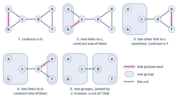
Repetition raises confidence but proves nothing. No run can tell whether its cut is the smallest one, so there is no certificate. That is the price of giving up flows.