3 Strings
Call me Ishmael.
Herman Melville, Moby-Dick (1851)
3.1 How did that line go?
Leo is the life of the party. Somebody tells a story about a disastrous first date, and before the laughter settles Leo adds one line from a film everybody at the table has seen, and suddenly the story is bigger than itself. The line carries that whole film with it: the scene, the actor’s face, the night each of them first watched it. For a moment the table is in sync: everyone is inside the shared experience, feeling part of something, understood. A good quote does that. That is Leo’s gift, and it is why he is invited everywhere. He never looked anything up. He just had the line.
Lately Leo’s memory is slipping. There is simply too much now: ten years of series watched late at night, podcasts on the way to work, films half-seen on planes, songs he never chose to learn but knows by heart. What used to fit on one shelf has become a flood, far more than anyone can keep track of. The lines are still in there, but they surface in pieces: a word, a rhythm, the place it fell in a scene. But a quote has to arrive in time. A minute late, the right line is just a man reciting; the moment it belonged to is gone. More than once the perfect line has come to him on the way home, word for word, with nobody left to say it to. It doesn’t count. A nearly right quote is no better: it ruins the moment, someone corrects him, and everyone laughs at him instead of with him.
Tonight the conversation has turned to something a book he loves has already put into words. There is a line for exactly this moment. Leo can feel its shape: something about November, something about weather inside a person. He can’t say it. He knows roughly where it lives, near the beginning of Moby-Dick, a few sentences after the three words everybody knows.
So he reaches under the table for his phone. The whole novel is there, free, about 1.2 million bytes of it, and he types the fragment he’s surest of into the search box: drizzly November. A pause, and there it is: “whenever it is a damp, drizzly November in my soul.” He says it, and it lands.
That pause is what this chapter is about. Leo’s phone just read the novel, all of it: it went through the text from the first character, lining his fragment up against it, until the characters agreed. Ask again a minute later, about a different line, and it reads the whole novel again from the start. Nothing it did the first time helps it the second.
There is an older way to find things in a book, and it fails in the opposite direction. The index at the back is built once and answers instantly forever after: look up whale, and there are the pages. But somebody built it by hand, it covers only the words an editor chose to include, and it runs for pages. Nobody indexes drizzly. A search engine does: it builds the same kind of list by machine, for every word of every page. That list is an inverted index. That finds drizzly, and drizzly November as a phrase. It still can’t find a piece of a word, like zzly Nov, because it knows only the words it cut the text into.
One way re-reads everything every time. The other answers at once, but only what someone thought to include, and it takes up room doing it. Each idea in this chapter fixes what broke in the one before. The chapter starts by making the reading itself cheaper. Then it prepares the text once, for fragments from the start of a quote, then for fragments from anywhere. Each preparation is bigger than the one before, until the index is larger than the book it indexes. The final one is an index that is smaller than the book, so complete that you could delete the book and still read any line of it back out of the index.
Leo’s phone held one novel. The ten books this chapter’s code was tested on hold nearly seven million bytes of text.1 A service that answers “where is this line from?” for everyone holds every book, script and lyric anyone can quote: Leo’s whole flood, and everyone else’s. That service is what makes each idea below necessary.
3.2 Reading the whole book, every time
Scanning and rolling fingerprints
Start with the plain way, the one Leo’s phone used. The text has \(n\) characters and the fragment, the pattern, has \(m\). Lay the pattern against the text at position 0 and compare character by character. The first time two characters differ, stop, slide the pattern one place to the right, and start comparing again. If you get through all \(m\) characters without a difference, you’ve found it. Every placement of the pattern is called a window of the text: the \(m\) characters it covers.
The text is abababababab and the pattern is ababc. Slide the pattern along by hand and count every single character comparison you make before you can say not found. Then say what the worst case costs in general, for a text of \(n\) characters and a pattern of \(m\), and point at the characters you compared more than once.
Five minutes, with a pencil. You’re done when you have a count for this text, a formula for the general case, and one character you can show was read at least twice.
3.2.1 Sliding a window
Count it on that text. At position 0, abab agrees and c does not: five comparisons. Slide one place: b against a, one comparison, out. Slide again: four agree, the fifth fails, five more. The pattern alternates between failing at once and failing at the last moment, and the windows that fail late cost the full five. By the end you’ve made 24 comparisons against a text of twelve characters, and most of those characters were looked at several times.
In the worst case every window is compared all the way to its last character, so the scan costs about \(n \times m\) comparisons. A pattern of twenty characters against the ten books comes to over a hundred million. And the waste has a precise shape: each window shares all but one character with the window before it, and the scan throws all of that away and starts again.
A five-letter pattern, a text of millions of letters, and comparing letter by letter at every position is too slow. Design something that dismisses almost every position with a single comparison, and still never misses a match or reports a false one. Go in two steps.
First, pretend each letter is a digit, so a five-letter window is a five-digit number. The window 17676 slides one place to 76764. Get 76764 from 17676 using only the digit that leaves and the digit that enters. Windows of twenty letters make numbers too big to handle in one step: what small number could you keep instead?
Then write down what must always be true of that small number, and what breaks without each one.
Ten minutes. You’re done when you have three or four invariants, and for each one, what goes wrong without it.
Look at your list. Did one of your invariants say what happens when two different windows get the same small number?
3.2.2 A number for each window
Suppose every character were a digit. Then a window of five characters would simply be a five-digit number, and comparing a window with the pattern would mean comparing two numbers: one step, not five. Better still, sliding the window would be arithmetic. The window 17676 becomes 76764 by removing the leading 1 (subtract \(1 \times 10^4\)), shifting what’s left one place (multiply by 10), and adding the new last digit, 4. Three operations, however long the window is.
But a window of twenty digits is a twenty-digit number, too big to handle in one step. So keep only the remainder after dividing by some fixed number, the modulus. The remainder is small whatever the window’s length, and the three-step slide still works on remainders, because subtracting, multiplying and adding all survive taking remainders along the way. That remainder is the window’s fingerprint⬢.
Here it is with real numbers, on a made-up text that starts with that same window: the nineteen digits 1767640259219659478. The pattern is 40259, and the modulus is 13. These are small enough to follow by hand. The real search, further down, uses every byte value as a digit and a modulus far larger, chosen at random. Write \(x \bmod 13\) for the remainder of \(x\) divided by 13. The first window has fingerprint \(17676 \bmod 13 = 9\), and a leading digit weighs \(10^4 \bmod 13 = 3\). So one slide is:
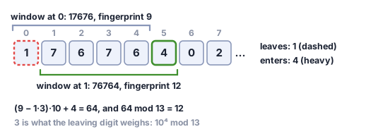
That is \((9 - 1 \cdot 3) \cdot 10 + 4 = 64\), and \(64 \bmod 13 = 12\). From scratch, \(76764 \bmod 13 = 12\) too. That has to happen every time: the slide never drifts away from the true fingerprint, however many times you repeat it.
Now roll it all the way across. The pattern’s own fingerprint is \(40259 \bmod 13 = 11\), so a window needs a closer look only when its fingerprint is also 11.
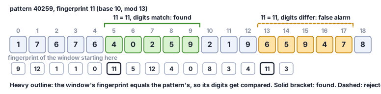
Fifteen windows, fifteen fingerprints, and two elevens. The window at position 5 is 40259, the pattern itself. The window at position 13 is 65947, which is nothing like it, and still has fingerprint 11.
3.2.3 When two numbers agree by accident
Look again at that second eleven. Thirteen remainders are possible, so plenty of different windows must share each one, and a fingerprint match only says maybe. The fingerprint is a fast filter that tells you where it makes sense to check. So every time two fingerprints agree, the search goes back and compares the actual characters, and only reports a position when they really match. At position 13 they don’t, and that window is thrown out: a false alarm, or spurious hit, caught.
That one comparison is what makes the method exact. A false alarm costs a wasted check, never a wrong answer, whatever modulus you pick. The modulus decides only how often the check is wasted. With 13 that is often, which breaks the design’s assumption. A large modulus picked at random⬢ restores it (the box below).
The three-step slide keeps the number equal to the current window’s without rereading the window (invariant 2), and the check reports nothing unchecked (invariant 3).
Roll it yourself below. Step through the windows one at a time. Then, before you change the modulus, guess: will 7 give more false alarms on this text than 13, or fewer? And 101? Change it, and watch how often the fingerprints agree by accident.
This is the Rabin–Karp search [1]. The code printed in this chapter follows the Python in the book’s companion library, algodesign, which also holds a Rust version built for speed. It is printed with a note beside each line or group of lines. Read down the code first, on its own, then come back for the notes. Where a listing keeps only the heart of a function, ... stands for the lines left out, and a link leads to the whole function in the library. Here is the search’s main loop.
In that code, text and pattern are bytes, so text[i] is already a number from 0 to 255, and a base of 256 makes every byte one digit. The slide is the 64 mod 13 step from above, with high standing in for the weight of the leaving digit. The whole function, with the set-up and the two edge cases (an empty pattern is everywhere, a too-long one nowhere), is in the companion library, in rabin_karp.py. There base and mod are passed by name. Run it on the hand trace, with each digit’s value as one byte, base 10 and modulus 13, and it reports the real match at position 5 and drops the false alarm at 13:
from algodesign.strings.rabin_karp import search

text = bytes([1, 7, 6, 7, 6, 4, 0, 2, 5, 9, 2, 1, 9, 6, 5, 9, 4, 7, 8])
pattern = bytes([4, 0, 2, 5, 9])
print(search(text, pattern, base=10, mod=13))   # [5]
With a large prime modulus picked at random, the whole search is expected to take about \(n + m\) steps, plus a full comparison for each real occurrence. The box below says why.
With a small fixed modulus like 13, false alarms are common, which is why the design assumes a large random prime. A fixed modulus has a worse problem: anyone who knows it can write a text in which many windows have the pattern’s fingerprint. Then each of those windows triggers a full comparison, and the search is back to about \(n \times m\). It still gives the right answer. It just stops being fast.
The defense is to choose the modulus at random each time, from all the primes below a threshold, so nobody can aim at it. Motwani and Raghavan work out how big the threshold must be [2, Sec. 7.6]: for a text of \(N\) bits and a pattern of \(M\) bits, a prime drawn below about \(N^2 M \log_2(N^2 M)\) produces a false alarm anywhere in the text with probability only about \(1/N\). On any text: the randomness is in the prime, not in the text. This is the random prime the design assumes. So the expected cost of the whole search is about \(n + m\) steps, plus a full comparison for each real occurrence.
A method that is always right and leaves only its running time to chance is called Las Vegas. Skip the check, and this one becomes Monte Carlo: always fast, and now and then wrong.
In practice, the library caps the threshold at \(2^{61}\), so that every product fits in 128-bit arithmetic. For a text the size of the ten books, and any pattern longer than one byte, that cap is lower than the formula asks for, and the bound gets weaker than \(1/N\).
The guarantee has a price on ordinary text. On the ten books, with both in the library’s Rust, a plain scan that compares each window letter by letter is about 1.6 times faster than Rabin–Karp.2 In English the first letter of a window almost always differs from the pattern’s, so the scan usually stops after one comparison, while the fingerprint does its arithmetic at every step. The scan’s cost climbs only where every window almost matches: for a long run of as searched for 255 as and a b, the two draw level. The fingerprint wins outright when many patterns of one length are searched at once, with all their fingerprints in one set.
Searching with borders: Knuth–Morris–Pratt and Aho–Corasick
Fingerprints are one way to stop re-reading the text. There is another, which uses no randomness at all: let the pattern’s own shape tell you how far to slide.
Say the pattern is ababc, and the text has just matched abab before failing. You don’t have to start again from scratch, because you already know what the text just said: it ended in ab, and ab is also how the pattern begins. So slide the pattern until its opening ab sits on top of that ab, and carry on comparing from there. A piece shorter than what you have matched that is both its start and its end is called a border. Work out the longest border of every beginning of the pattern once, before the search, and keep them in a table, the prefix function. Then the search never has to step back in the text. The whole job takes a number of steps proportional to \(n + m\), guaranteed, on every text, with no false alarms to check. Searching this way is the Knuth–Morris–Pratt method [3].
Dice make the method simple and fast on average, for every text, as long as nobody can guess the prime. The pattern’s structure makes the guarantee hold every single time, at the price of a trickier method.
Borders also work for thousands of patterns at once. Store the patterns in a tree that keeps their shared beginnings once, the trie of the next section. Give each node a link to where to carry on when the next letter fails: the longest piece, shorter than what has matched, that ends it and begins one of the patterns. That is a border, worked out across all the patterns. Then one pass over the text finds every pattern in it. That is the Aho–Corasick method [4], and building it lies beyond this chapter.
Many standard libraries search without dice, with a relative of Knuth–Morris–Pratt called Two-Way [5], among them glibc’s memmem for patterns over 256 bytes and Rust’s str::find. For patterns of 3 to 256 bytes, memmem uses a method from the Boyer–Moore family [6], [7]: it reads the last letters of each window first, and when they cannot end a match, it jumps ahead by up to the whole length of the pattern. Patterns of one and two bytes get a search of their own.
3.2.4 Too much to read
Rolling fingerprints make one search cheap: one pass over the text, a few arithmetic steps per window. But one pass is still a pass over everything, every time anyone asks.
GitHub worked through exactly this arithmetic when it rebuilt its code search [8]. The code it wanted searchable came to about 115 TB. Scanning that much with one of the fastest scanning tools there is, perfectly spread over 2048 processor cores, would take about 96 seconds per query, with every core busy, so the whole system could answer about one query every hundred seconds. Their conclusion is the one this chapter reaches next: “we need to build an index.” With the code stored inside it, their index came to about 25 TB, about a fifth of the original.
An index is the other road from the start of the chapter: read the text once, before anyone asks, and keep something that lets each question touch only a small part of it. What to keep depends on what Leo remembers, and the simplest case is a quote’s start.
3.3 I remember how it starts
Trie and Patricia tree
A week later, another dinner. Somebody is describing their sister’s wedding, the speeches, the mother-in-law, and Leo knows there is a perfect opening line for it, the famous first sentence of Pride and Prejudice, a novel about marriage and money. He has the start of it: “It is a truth…” And then nothing.
This time the fragment he holds is a beginning, and you do something with beginnings many times a day without thinking about it. Type the first letters of a name into your phone’s contacts, or the first word into a search box, and the list below narrows with every letter you add. Nobody is reading every entry from the start each time you press a key. The list is ready for exactly this question, what starts like this?, before you ask it.
You want to store a few thousand quote openings so that typing the first words lists every opening that begins that way, with the list narrowing as you type. A sorted list and binary search, from the search chapter, would find the matching block. But look at the openings themselves: “It is a truth”, “It is a far, far better thing”, “It was the best of times”. What do they share, and could your structure store the shared part only once? Design it, and say what one keystroke costs.
Ten minutes. Draw your structure for the five words she, shells, sea, shore, seashore. You’re done when you can count how many pieces your drawing uses, and say how much work typing one more letter takes.
3.3.1 A tree of first letters
Look at what your drawing did with she and shells. Did it store she twice, or once, with lls hanging off its end? The three openings do the same: all three share “It”, and two of them share “It is a”.
Start with one empty node, a point that branches will hang from: the root. To store a word, walk down from the root one letter at a time: if there is already a branch for the next letter, follow it; if there isn’t, make one. When the letters run out, mark the node you stand on: a word ends here. That’s the whole structure, and it is called a trie, from retrieval [9].
Here are the five words, stored that way.
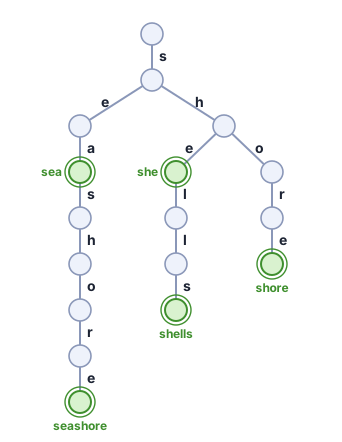
No node in the picture holds a word, or even a letter. The letters live on the branches, and a word is nothing but the path you walk to reach its ring. she and shells share their first three branches; shells just keeps going. Seventeen nodes are enough for all five words, root included.
The order the words arrive in makes no difference: the same words always build the same tree. The search chapter’s trees could not promise that, and needed rules to stay balanced. A trie never needs them, because its depth is the length of its longest word.
The design’s first invariant is the whole of search: follow the letters, and the mark answers. The second is why there is only ever one way to follow them.
Here is the insert in code. Each node keeps its children in a small dictionary, filed by the next byte, and a flag that says whether a word ends there. A node where a word ends also keeps whatever is stored with it, its value. _Node() makes an empty node, and every walk starts at self.root.
Finding a word is the same walk without the building: follow the branches letter by letter, and check the flag where you stop. Count what that costs. Every step uses one letter of the word you are looking for, so a word of \(m\) letters takes \(m\) steps, however many words are stored. A thousand openings or ten million, typing one more letter is one more step down. Binary search over a sorted list cannot say that: its number of steps grows with the size of the list.
3.3.2 Everything that starts with…
Now Leo’s question. Walk down the letters he remembers, and stop. Every word that starts that way is below the node where you stopped, and nothing else is. So the answer is that one branch, read off from the top. The walk down is the walk that finds a word, so the code below (Listing 3.4) is only the reading off. It starts at the node where the walk stopped, with path the letters that led there, and puts every word it meets into the list out.
Try it on the picture. For sh, walk s, then h. Below that node sit she, shells and shore, and nothing else, because every other word went another way at the first branch. For se, the answer is sea and seashore. For x, the walk fails at the first letter, and the answer is empty immediately, without looking at a single stored word.
The answers come out in byte order for free, which for lowercase words like these is alphabetical order. _collect visits a node before the nodes below it and takes the branches in order of their letters. That is exactly byte order, in which a word comes before every longer word it begins. The whole of keys_with_prefix, walk included, is in the companion library, in trie.py.
A careless remove breaks invariant 3: it clears a word’s mark and leaves the branch that spelled the word, now leading to no word at all. The library’s check_valid() returns None when every invariant holds, and otherwise names the first one that fails, numbered as in the box:
from algodesign.strings import Trie

trie = Trie()
for word in [b"tea", b"ten", b"to"]:
    trie.insert(word, len(word))
print(trie.check_valid())      # None
node = trie.root
for byte in b"to":
    node = node.children[byte]
node.has_value = False         # clear the mark, keep the branch
print(trie.check_valid())      # invariant 3 (no_dead_branches)
3.3.3 When the tree is bigger than the words
The five words have 25 letters between them, and the trie spends 17 nodes on them. That sounds reasonable until you ask what a node costs.
The fast version of this structure, the one in the library’s Rust, gives every node one slot for every possible next byte, 256 of them, so that following a branch is a single lookup with no search at all. Each slot is a pointer of 8 bytes, so a node is about 2 kilobytes. Seventeen nodes come to about 35 kilobytes, to store 25 bytes of words. The Python above saves the empty slots by using a dictionary, but every entry in a dictionary has its own cost, and the shape of the waste is the same.
That shape is the long chains. Look at seashore: after sea come four nodes in a row that each have exactly one child and hold no word, there only to spell out s, h, o, r before the e where seashore finally ends. One node per letter, and nothing to choose at any of them. The same happens to shells after she, and to shore after sh. A trie is small when its words share a lot. When they mostly don’t, it is mostly chains, and every link of a chain is a node paid for in full.
3.3.4 Squeezing the chains
So squeeze them. Wherever a node has exactly one child and no word ends at it, merge it with that child, and write the merged letters on the branch: one branch labeled shore instead of five branches labeled s, h, o, r, e. The result is called a Patricia tree [10]. A compressed trie like this is also called a radix tree, where radix is the number of different digits a key is written with: 2 for bits, 256 for bytes, 26 for lowercase letters.
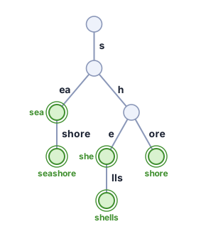
Eight nodes, and the picture says why: every node below the root now ends a word or branches⬢, as the design’s third invariant asks.
Keeping it pays off: such a tree has at most two nodes for every word stored, however long the words are. The root is the one exception. It has nothing above it to merge into, so it may keep a single child, as it does here, where every word starts with s.
Say the tree stores \(k \ge 1\) words. Its nodes come in three kinds. There is the root. There are the nodes below the root where a word ends: at most \(k\) of them, one for each word. And every other node below the root ends no word, so by the third invariant it branches: it has two children or more.
Count that last kind. Every leaf ends a word, so there are at most \(k\) leaves. And in any tree, the nodes with two or more children are fewer than the leaves: a single path down ends in one leaf, and every split adds at least one more leaf. So at most \(k - 1\) nodes branch without ending a word.
All together, at most \(1 + k + (k - 1) = 2k\) nodes, however long the words are.
Invariants like these only help if they stay true after every change, which is where the work is. Inserting walks down whole branch labels while they agree with the new word, and ends in one of three ways:
- the word runs out exactly at a node: mark it;
- no branch starts with the next letter: hang the whole rest of the word on one new branch;
- the word agrees with a branch for a while and then disagrees in the middle of its label: split the branch at the point of disagreement, so the branches leaving a node still start with different letters (invariant 2).
To see the third, insert she, then shells, then sea:
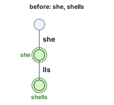
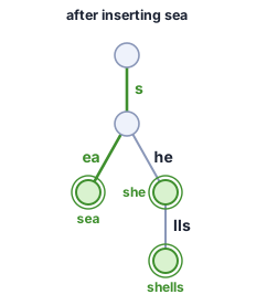
she agreed with sea for one letter, so it splits after s. The new node and the new branch are drawn heavy.
sea agrees with the branch she for one letter, s, and then the two part. So the branch is cut after s: a new node goes there, the old branch keeps the rest of its label, he, and sea’s own remainder, ea, hangs beside it. The new node branches, so every node still ends a word or branches (invariant 3).
In the code, each node keeps the label of the branch that leads into it, and _Node(label) makes an empty node with that label. _leaf(rest, value) makes a node that ends a word, with rest as its label, and _common_prefix_len(label, rest) counts the letters the two agree on from the start.
Taking a word out runs the same rules the other way. Clear the word’s mark, then remove any node left with no word and no children, walking back up. In the squeezed tree, that can leave a node with a single child and nothing else to do, and it is merged with its child at once, so every node again ends a word or branches (invariant 3).
The Python above files each branch in a dictionary under its first letter. The library’s Rust keeps each node’s branches in a list sorted by first letter, and picks one by binary search.
Try both structures below. Insert words of your own and watch where the branches split, switch the squeezing on and off and compare the node counts, and remove a word to see a chain merge back together.
3.3.5 What a beginning can’t do
Leo, with his trie, finds “It is a truth universally acknowledged” in a few keystrokes. But a trie answers only the question it was built for. It needs the start. Give it “universally acknowledged”, the part he actually remembers most nights, and it has nothing to offer: every path in it begins at the first letter of a stored opening, and that fragment is no opening.
Asked a slightly different question, the same structure is also one of the ways a router decides where to send each packet it receives. The router appendix at the end of the chapter shows how.
3.4 It was somewhere in the middle
Suffix array and LCP
Most nights, the middle is all Leo has: “…universally acknowledged…”, two words and a rhythm, with no idea what came before them.
The index at the back of a book has the same blind spot from another side. It lists the words an editor expected someone to look up, and nobody expects anyone to look up universally. What Leo needs is an index that can be entered from anywhere: from any word, from the middle of a word, from any position in the text at all.
You want an index over a text of \(n\) characters that finds any fragment wherever it sits, not only at the start of a line. Take the six-letter text banana. Every fragment of it starts at some position. Before building anything, write down what must always be true of your index. Then: what would one entry of it be, how many entries are there, and how many bytes does the whole index take for a text of \(n\) characters?
Ten minutes, with the word banana. You’re done when your invariants guarantee that no occurrence is missed and that finding one leads to the rest, you have written your index for banana, found ana in it by hand, and put a size in bytes on it for a text of \(n\) characters.
3.4.1 Every fragment starts a tail
Look at your index for banana. If each entry held a fragment’s letters, how many entries did you need, and how long were they? Now count something smaller: how many places can a fragment start?
A fragment of the text starts somewhere, and from that position the text runs on to its end. That tail, from some position to the end, is called a suffix. ana occurs at position 1 of banana, which says exactly this: the suffix starting at position 1, anana, begins with ana.
So finding a fragment anywhere in the text is the same as finding a suffix that begins with it. Write the text with a $ at the end: a marker, called a sentinel, that means the text stops here, and that sorts before every letter. In the library, $ is byte 0, which no text holds, so a dollar sign in a book is just another letter. The sentinel stops one suffix from being the start of another.
The last section’s trie answers exactly what begins like this?, so put every suffix into one. It works: walk the fragment’s letters from the root, and the suffixes below that point are its occurrences. But it does not fit. Two suffixes of ordinary prose share only a few letters before they part, so nearly every suffix lays down its own chain to the end of the text: about \(n^2/2\) nodes, well over 700 billion for Moby-Dick. Squeezing the chains, as the Patricia tree did, gives the suffix tree [11], [12], [13], about 1.4 nodes per letter on ordinary prose (Project 9 measures it). But each node must point into the text for its label and link to its children, about 24 bytes a node, so the index takes some 34 bytes for every byte of book, and the book must be kept beside it. For Leo’s flood that is far too much. What is needed is less: only where each suffix starts.
3.4.2 Keep where it starts, not what it says
Step back and ask what that tree gives you. A trie keeps its branches in letter order, so reading the suffixes off it from left to right gives them in alphabetical order.
So keep only the order. Sort the suffixes (invariant 2), and for each one store just one number: the position where it starts, each position once (invariant 1). The letters are already in the text; there is no need to copy them.
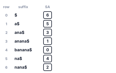
banana$ sorted this way is the array 6 5 3 1 0 4 2: seven numbers for seven characters. This is the suffix array [14]. In Python, the suffix array is sorted(range(n), key=lambda i: text[i:]): the start positions, sorted by the suffix that starts at each. Any faster way to build it must give exactly this.
Each sorted suffix sits in its own row of the table, numbered from 0 at the top: row 0 is $, row 4 is the whole text. From here on, a suffix is named by its row. Whenever a search needs the letters of the suffix in some row, it looks them up in the text, starting at the number stored there. One number per character, and every fragment of the text has a row whose suffix begins with it.
3.4.3 Searching the sorted suffixes
The array is sorted, so the search chapter’s binary search applies, with one twist: it compares the pattern against just the first few letters of a suffix, as many as the pattern has.
Find ana. The rows whose suffixes begin with ana form one stretch, so the search looks for its top and its bottom. For the top, it halves toward the first row whose first three letters do not come before ana in sorted order. It looks at row 3 (ana, not before, so the top is at row 3 or earlier), then row 1 (a$, before ana, so the top is after row 1), then row 2 (ana, not before). The top is row 2. The bottom is found the same way, as the first row whose first three letters come after ana: row 3 (ana, not after), row 5 (na$, after), row 4 (ban, after). The bottom is row 4, just past the stretch, so the stretch runs from row 2 up to, but not including, row 4: rows 2 and 3, holding positions 3 and 1. Six looks at the array find the stretch of every occurrence.
In code it is shorter than the explanation, because Python’s bisect does the halving and key cuts each suffix down to the pattern’s length.
Count what that costs. Each look is a jump to a random place in the text, a fetch in the search chapter’s terms. It compares at most \(m\) characters there, and each of the two searches takes about \(\log_2 n\) looks. The ten books from the start of the chapter hold 6,793,686 bytes, so each needs at most 23 looks. For “universally acknowledged”, 24 characters, that is at most 46 looks of at most 24 comparisons each: about a thousand character comparisons, where the scan of the first section compared against every one of almost seven million windows.
And Leo’s two words come back with two answers. One is the line he was looking for, the first sentence of Pride and Prejudice. The other is in Great Expectations, where a small-town newspaper praises “our as yet not universally acknowledged townsman TOOBY, the poet of our columns”. Perhaps Dickens had read Austen; two words can’t tell.
Build an array yourself below, then search it, one look at a time.
3.4.4 Sorting by doubling
Leo never sees this part. The service does, once for every book it holds. Searching was easy because the hard work was done in advance: the suffixes had to be sorted. Hand them to any sort, and each comparison between two suffixes reads letters until they differ. In ordinary prose that is quick. In a text with long repeats it is not: in a text of a million as, every pair of suffixes agrees until one of them runs out, and the sort spends most of its time re-reading the same letters.
The way out is the same move the fingerprints made in the first section: stop comparing letters, and compare small numbers that stand for many letters at once.
Start by giving each position a tag, a number that sorts the suffixes by their first letter alone, with equal letters getting equal tags. In banana$, $ gets 1, every a gets 2, b gets 3, every n gets 4.
Now the step that repeats. Suppose the tags sort the suffixes by their first \(w\) letters, and two suffixes share a tag exactly when those letters agree. The first \(2w\) letters of the suffix at position \(i\) are its own first \(w\) letters, then the first \(w\) letters of the suffix at \(i + w\). Both already have tags. So the pair (tag of \(i\), tag of \(i + w\)) sorts the suffixes by their first \(2w\) letters, without looking at a single letter. Sort the pairs, hand out new tags, and the prefix each tag covers has doubled [15, Sec. 32.5]. A suffix that would start past the end of the text gets tag 0, smaller than every other, because a suffix that runs out sorts first.
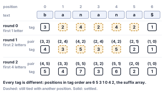
Follow position 1 through the figure. Its first letter is a, tag 2. In round 1 its pair is (2, 4): its own a, then the n at position 2, so it is tagged by an. In round 2 its pair is (3, 3): an, then the an at position 3, so it is tagged by anan. By then every position has a tag of its own, and reading the positions in order of tag gives 6 5 3 1 0 4 2. That is the suffix array, and no two suffixes were ever compared letter by letter.
Each round sorts the pairs in two passes of counting sort, the kind that keeps equal keys in the order they arrived: first by the second tag, then by the first. Because the second pass keeps ties in the order the first pass left them, the pairs come out sorted by first tag, then second. The prefix a tag covers doubles every round, so for a text of \(n\) characters it takes about \(n \log_2 n\) steps at most.
It usually stops much sooner. The tags become all different as soon as that prefix is longer than the longest passage that occurs twice in the text. That passage, in the ten books, is 145 bytes long, so the prefix stops at 256 letters, after 8 rounds, not the 23 that \(\log_2 n\) allows.
Faster constructions exist. DC3 [16] and SA-IS [17] build the suffix array in a number of steps proportional to \(n\), and libraries built for very large texts use methods of their kind.
Why two old tags are enough: the appendix. The code that sorts the pairs in two counting passes, with its tests, is in the companion library, in suffix_array.py.
3.4.5 Neighbors that agree
The sorted order holds one more thing for free. Look at any two neighboring rows: they share some opening letters, then part. ana$ and anana$ share ana, three letters. na$ and nana$ share na. Write down, for each row, how many letters its suffix shares with the row above, and you have the LCP array, for longest common prefix. For banana$ it is 0 0 1 3 0 0 2.
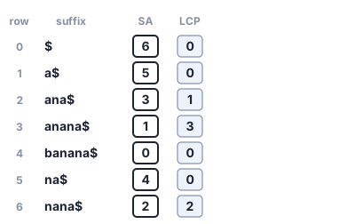
That array answers a new question in one pass: what is the longest passage that occurs twice? A passage that occurs twice starts two suffixes that share it, and suffixes that share a long opening sort close together. So the largest number in the LCP array is the length of the longest repeat, and the row where it sits says where. In banana$, the 3 in row 3 is ana.
In the ten books, the largest entry is 145 bytes, and the passage it points to is two lines from Alice’s Adventures in Wonderland, the chorus of the Mock Turtle’s song:
Will you, won’t you, will you, won’t you, will you join the dance?
Will you, won’t you, will you, won’t you, won’t you join the dance?
Both lines together appear in two verses. Nothing else in almost seven million bytes of Austen, Melville, Dickens, Shelley, Stoker, Doyle, Wilde, Twain and Carroll repeats for longer.
Computing each entry from scratch means comparing two suffixes letter by letter, and in a text full of repeats that is slow again. But the whole array can be computed in one pass, in time proportional to \(n\), by walking the suffixes in text order, not sorted order, and carrying the count of matching letters from one suffix to the next. This is Kasai’s method [15, Sec. 32.5], [18].
Kasai’s method step by step, and why the count drops by at most one: the appendix. Its code, with its tests, is in the companion library, in lcp.py.
3.4.6 How big is the index?
Add it up. The text is \(n\) bytes. The suffix array holds one number per character, and a 4-byte number per entry is enough for any text up to about 4.29 billion characters. Together that is \(5n\) bytes: five times the book. For the ten books, about 34 MB to search 6.8 MB of text. Past about 4.29 billion characters each entry needs more than 4 bytes, and with 8-byte numbers the index grows to \(9n\). Keep the LCP array as well, and add another \(4n\). Even then it is far below the suffix tree’s 34 bytes for every byte of book, with the book kept beside it. And it gives up none of the tree’s answers: with the LCP array and a little more bookkeeping, any algorithm written for the suffix tree can run on the sorted order instead, just as fast [19].
Language models learn from text cut into pieces called tokens. In 2024 a suffix array of this kind was built over five trillion of them, and it counted in milliseconds how often any phrase appears [20]. But it pays the same price at every scale: the index is several times bigger than the text, and the text must be kept beside it, because every comparison reads it.
Leo’s flood is every book, script and lyric anyone can quote. Five times that, or more, is a lot of disks to answer a question at dinner.
3.5 What is this all about?
Text indexes: count, locate, extract
Step back from fingerprints, trees and sorted suffixes for a moment. Under all of them, Leo has been asking the same three questions, and every structure so far answers them differently:
- Is that really the line, and how often does it come up? Whether the fragment occurs in the text, and how many times. (
count) - Where is it? The positions where it occurs, which say which book and which page. (
locate) - Give me the words. The text around a position, so he can say the whole line. (
extract)
A structure that answers those three questions is a text index, and the questions are not only about quotes. A plagiarism checker asks whether a student’s sentence occurs in a pile of published work, and where. GitHub’s code search, from the first section, asks where a line of code occurs across millions of repositories. A DNA sequencer produces short pieces of DNA, called reads, and each one has to be placed on a reference genome three billion letters long. Covering every letter about thirty times over, at 150 letters a read, takes about 600 million of them. And when a language model writes a paragraph, someone eventually asks whether that paragraph was copied from what it was trained on: count, locate, and show me. Same three questions, every time, and the same tension between preparing the text once and answering fast.
3.5.1 What is a character, actually?
Under the three questions sits a fourth, older one: what counts as the fragment? Leo’s drizzly November worked. Try another line from the same chapter of Moby-Dick, “growing grim about the mouth”, and search the ten books for it. Nothing. The quote is there. But the file starts a new line after about, so the byte between about and the is a newline, not a space, and the search compares bytes.
It gets worse with apostrophes. Search the same ten books for don't, typed with the apostrophe on your keyboard: zero hits. Search for don’t with the curly apostrophe the books were typeset with: 1085. The two look nearly the same on screen but are different bytes in the file: the curly one is the three bytes e2 80 99 (in hexadecimal), the keyboard one is the single byte 27. The search is not wrong. It found exactly what it was asked for, and what it was asked for was not what you meant.
Everything in this chapter treats text as a row of bytes, and compares bytes. That is a choice, and it has costs:
- One letter can be written in more than one way.
éis stored either as one character or asefollowed by a combining accent, and the two forms compare unequal even though they look identical. - What you see as one letter can be several characters. A flag or a family emoji is a short run of characters that the screen draws as one symbol, so counting “letters” depends on who is counting.
- “Sorted” depends on the language. Alphabetical order is a convention, and different languages have different conventions, so the order of words is not a property of the bytes alone. The suffix array you just built sorted bytes, and nothing else.
Fixing these is a separate job, done before the search ever sees the text: rewrite every character into one agreed form, and decide which differences count. The code in this chapter does none of that, on purpose. It answers exactly what it is asked, and deciding what to ask stays with you.
3.5.2 What has been bought so far
Here is the ledger, for a text of \(n\) characters and a fragment of \(m\):
| structure | prepare | answer one fragment | size | which fragments |
|---|---|---|---|---|
| Scan, with rolling fingerprints | nothing | about \(n + m\) steps, expected, plus \(m\) per occurrence | the text | any |
| Trie, Patricia tree | build once | \(m\) steps, plus the answers | a node per letter, or per branch, of the stored openings | beginnings only |
| Suffix array | sort once | about \(2m \log_2 n\) comparisons | \(5n\): the text plus the array | any |
The pattern across the table is the same one the search chapter found: what a structure wins in one column, it pays for in another. The suffix array answers any fragment fast, and pays for it in space.
Look at one more thing the three rows share. In every one of them, the text is kept, whole and untouched, and the answers depend on it: the scan compares against it, the trie was built from copies of it, the suffix array reads it on every comparison. extract has been free all along, because the text was sitting right there.
3.6 Useful mess?
Burrows–Wheeler transform
What if the text were rearranged, kept at exactly its own size, into an order that does the index’s job, and nothing were lost?
Here is a way to do it by hand. Take the text banana$ and write out all seven of its rotations: the text, then the text with its first character moved to the end, and so on (banana$, anana$b, nana$ba, …). Sort the seven rows, $ before every letter. Now keep only the last character of each sorted row, top to bottom. You get annb$aa.
Suppose all you were given was annb$aa, and the rule that made it. Could you get banana$ back? Start with this: what do you know about the first character of every sorted row, if you know the last ones?
Fifteen minutes. You’re done when you have recovered the first two characters of the text, or can say exactly what stops you.
The column you just made has a name: the Burrows–Wheeler transform⬢ of the text, BWT for short [21]. Here is the design behind it; check your answer against it.
Before seeing how to undo it, look at what it is.
3.6.1 Sort the rotations
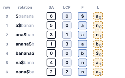
$, around to the start of the text (the gray letters), so every row is a rotation, and the rows are the seven rotations of banana$, sorted. The first column, F, is the text’s letters in sorted order. The last column, L, is the transform. Each row’s last letter comes, in the text, just before its first letter. The small number on each letter of L says how many copies of that letter sit above it in L, counting from 0; the next section uses them.
Leo’s lines come back in pieces and out of order, and he still knows they are all in there. The last column keeps every letter, only in another order.
Two columns matter. The first, F, is just the text’s letters sorted: $aaabnn. The last, L, is the transform: annb$aa. And because every row is a rotation, a row’s last letter is the one that comes, in the text, just before its first letter, wrapping around from the end to the start. Row 2 is ana$ban, and its last letter, n, comes just before the a at the start of ana$ in banana$.
The rows of the sorted rotations are almost the sorted suffixes of the suffix array. Cut each rotation at the $ and you get a suffix, and because $ is unique and smaller than every letter, the cut never changes the order. So row \(i\) is the suffix the suffix array stores in row \(i\), and the transform needs no rotations at all: L[i] = text[sa[i] - 1], the letter just before each sorted suffix (at position 0, Python’s text[-1] wraps around to the $). That is how the library computes it, from the suffix array in one pass.
3.6.2 Reading it backwards
The question from the box is how to get the text back from annb$aa alone.
The first step is the one you probably found. Sorting annb$aa gives $aaabnn, which is F: the first column is the text’s letters in sorted order, and the transform holds exactly the text’s letters (invariant 1). Now every row gives a pair, last letter then first letter, and each pair is two consecutive characters of the text, reading around from its end to its start: a$, na, na, ba, $b, an, an. Sort those pairs and you have the first two columns of the matrix. Put the last column in front of them again and sort, and you have the first three. Repeat, and after \(n\) rounds the whole matrix is back, and the text is the row that ends in $: the transform alone rebuilt it (the design’s promise).
That works, and it costs \(n\) sorts of \(n\) rows. The faster way rests on one fact about equal letters.
There are three as in each column. Number the copies of each letter down the column, starting from 0, and write the number small beside the letter. In L, a0 is in row 0, a1 in row 5 and a2 in row 6. In F, a0, a1 and a2 are in rows 1, 2 and 3. The number is how many copies of the same letter sit above it. a2 in L is the same character of the text as a2 in F, and so on for every letter and every number.
Here is why. The as in F are in sorted order of what follows them in the text, because that is the rest of their rows. The rows with an a in L are also in sorted order, and each of those rows, read from the start, is exactly what follows its a in the text. Same as, sorted by the same thing, so the same order.
as of banana$, in L and in F.
| copy | its row, with the a last in L |
its row, with the a first in F |
|---|---|---|
| a0 | row 0: $banan + a |
row 1: a + $banan |
| a1 | row 5: na$ban + a |
row 2: a + na$ban |
| a2 | row 6: nana$b + a |
row 3: a + nana$b |
Take the a off, and both columns hold the same three strings, $banan, na$ban and nana$b, in the same sorted order.
That gives a jump from any row to another, called the LF mapping, or LF, for last to first. From the row whose last letter is \(c_k\) in L, it jumps to the row whose first letter is \(c_k\) in F. Each row’s last letter comes just before its first, so the row you land on starts one position earlier: LF, read off L, the one column kept, walks the text backwards, one fetch per step.
The jump is cheap to compute. For each character \(c\), let C[c] be the number of characters in the text smaller than \(c\), which is the row where \(c\)’s block starts in F. Let occ(c, i), for occurrences, be the number of \(c\)s in L above row \(i\). For banana$, C is 0 for $, 1 for a, 4 for b and 5 for n. Then
\[\text{LF}(i) = C[c] + \text{occ}(c, i),\]
where \(c = L[i]\). For that \(c\), \(\text{occ}(c, i)\) is just the small number on \(L[i]\): row 1 ends in n0, and \(\text{occ}(\texttt{n}, 1) = 0\). And because the row you land on starts one position earlier in the text,
\[\texttt{sa}[\text{LF}(i)] = \texttt{sa}[i] - 1.\]
Row 1 holds position 5, and \(\text{LF}(1) = C[\texttt{n}] + \text{occ}(\texttt{n}, 1) = 5 + 0 = 5\). Row 5 holds position 4. The one exception is the row holding position 0, row 4: it jumps to row 0, which holds the $ at position 6, wrapping around to the end. Finding where a match sits, later in the chapter, rests on this line.
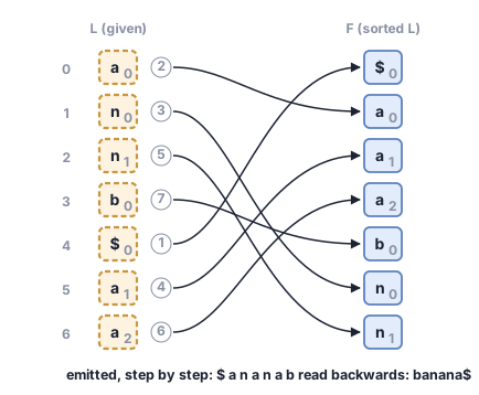
Walk it, reading the numbers off the figure. Start at the row whose last letter in L is $, row 4: that row is the whole text, banana$. Row 4 ends in $0: emit $. $0 heads row \(C[\$] + 0 = 0\). Row 0 ends in a0: emit a. a0 heads row \(C[\texttt{a}] + 0 = 1\). Row 1 ends in n0: emit n. n0 heads row \(C[\texttt{n}] + 0 = 5\).
Now take the last four steps yourself, from row 5, until you emit b.
Rows 5, 2, 6 and 3 end in a1, n1, a2 and b0, so you jump to \(1 + 1 = 2\), \(5 + 1 = 6\) and \(1 + 2 = 3\), and emit a, n, a, b. Seven steps, and the characters came out as $ a n a n a b, which is banana$ read backwards.
Here is the walk in code, with the LF of every row worked out first. The whole function, including the count that builds C, is in the companion library, in bwt.py.
Step the walk yourself below, and try the slow way, by sorting, beside it.
In this chapter’s construction, the marker $ has to be there, exactly once, and smallest. Without a unique end, the walk would not know which row is the whole text, and the rotations would no longer sort in the same order as the suffixes. The text abaa shows it: its rotations sort as positions 2 3 0 1 and its suffixes as 3 2 0 1, because a suffix that runs out sorts first while a rotation wraps around and keeps going. With $ at the end the two orders agree, and the library refuses any text that holds a second $.
3.6.3 It is not compression
The walk shows that the transform loses nothing. It saves nothing either: it has exactly as many characters as the text, and exactly the same ones. What it changes is order, and that order has a habit that becomes visible on real text.
The rows are sorted by how they begin, which is what follows each row’s last character in the text. So characters that come before similar contexts land next to each other. In English, what comes before he is most often t. Take Moby-Dick: of the 14,623 places where he occurs, 12,455 have a t in front of it. All those rows are neighbors in the sorted matrix, so their last characters form a long stretch of the transform that looks like this:
ttttttTttt tttttt tttttttttttt
The text itself never looks like that. The transform gathers letters that occur in similar company into runs, and a run like that is easy to squeeze by some later step that writes “t, twelve times” instead of twelve ts. That is how the bzip2 compressor uses it, and the compression chapter takes it from there. Repetitive collections often produce fewer, longer runs, and counting the runs gives another useful measure of their size.
Here, the transform has a different job. Seven shuffled letters and a table of four counts gave the whole text back, and that alone is a curiosity: the text, stored in a stranger order. The next section turns the same walk into an answer to Leo’s question.
3.7 By heart
FM-index and backward search
Picture the service that answers Leo’s question for everyone. It holds his whole flood, and everyone else’s: every book, script and lyric. At five times the text or more, its index is the biggest thing it owns. Now suppose it kept only the transformed column, the same size as the text, and threw the text itself away. Could it still find “universally acknowledged”?
You have only the last column of banana$, annb$aa, the table C (0 for $, 1 for a, 4 for b, 5 for n), and the fact from the last section: with the copies of each letter numbered from 0, \(c_k\) in L is \(c_k\) in F. No text, no matrix. Decide whether ana occurs in banana$, and how many times.
A hint for where to start: which rows of the sorted matrix begin with the last letter of the pattern?
Fifteen minutes. You’re done when you know which rows begin with a, and then which rows begin with na.
Look at your rows for na: did you find them from L and C alone, without the text? Here is the design your answer should match.
3.7.1 Searching backwards
Rows that begin with a are easy: they are a’s block in F, rows 1, 2 and 3. Write that as the stretch \([1, 4)\): from row 1 up to, but not including, row 4. Every step from here keeps the design’s invariant: the stretch is exactly the rows that begin with the part of the pattern read so far.
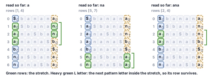
Now the pattern grows one letter to the left, to na. Which rows begin with na? Drop the n from such a row, and what is left begins with a, so it is one of rows 1 to 3. The question becomes: which of rows 1 to 3 has an n just before it in the text? The letter just before a row’s first letter is its last letter, in L. That is why the pattern is read from its end. Row 1, a$banan, ends in n. Row 2, ana$ban, ends in n. Row 3, anana$b, ends in b. Rows 1 and 2 end in n0 and n1, and the LF jump from the last section takes them to the rows that start with n0 and n1: na$bana and nana$ba, the rows that start one position earlier, with that n.
Where do the new rows sit in n’s block? Each n in L carries a number, and that number is its place in n’s block in F. The number on the first n inside the stretch is the count of ns in L above row 1, where the stretch starts. So that count is where the new rows start.
n lie in L above each row.
| row | L | \(\text{occ}(\texttt{n}, \text{row})\): how many copies of n lie in L above that row |
|---|---|---|
| 1 | n0 | 0 |
| 2 | n1 | 1 |
| 3 | b0 | 2 |
| 4, just past the stretch | $0 | 2 |
So the new stretch needs only two numbers: 0, the ns in L above row 1, and 2, the ns above row 4. Add each to 5, where n’s block starts in F, and the rows beginning with na are 5 and 6, na$bana and nana$ba. One more letter to the left, a, works the same way, from those two rows: L holds one a above row 5 and three above row 7, and a’s block starts at row 1. The whole search, one letter per line:
ana in banana$, one letter per line.
| letter read | lo | hi | rows | they begin with |
|---|---|---|---|---|
a |
1 | 4 | 1, 2, 3 | a |
n |
5 + 0 = 5 | 5 + 2 = 7 | 5, 6 | na |
a |
1 + 1 = 2 | 1 + 3 = 4 | 2, 3 | ana |
Each line adds two numbers: \(C[c]\), where the letter’s block starts in F, and how many of that letter lie in L above the old lo, or above the old hi. Written once, reading one more letter \(c\) to the left turns the stretch into
\[[\text{lo}, \text{hi}) \;\to\; [\,C[c] + \text{occ}(c, \text{lo}),\; C[c] + \text{occ}(c, \text{hi})\,).\]
The last line’s rows, 2 and 3, are ana$ban and anana$b. The answer to how many? is \(4 - 2 = 2\), and the text was never consulted.
Count the cost. Each letter of the pattern needs two counts, \(\text{occ}(c, \text{lo})\) and \(\text{occ}(c, \text{hi})\). That is two questions per letter, whatever the length of the text. If those two counts are fast, finding how often a 24-letter fragment occurs in one index, whatever its size, is 48 questions.
This is the FM-index, invented by Paolo Ferragina and Giovanni Manzini [22], and backward search is its central idea. The whole design now hangs on one operation, counting a letter above a row. Three jobs are left: counting it fast without keeping much more than the column itself, saying where each match starts, and reading back the words around it.
3.7.2 Counting fast
Counting the \(c\)s above a row one by one would be a scan of L again. Instead, keep checkpoints: every \(k\) rows, store how many of each letter came before that row. Then \(\text{occ}(c, i)\) is one lookup, at the last checkpoint at or before row \(i\), plus a short count of the \(c\)s between it and row \(i\). In one line:
\[\text{occ}(c, i) = \text{occ}(c, \text{checkpoint}) + c\text{s between}.\]
The \(c\)s between are counted from the checkpoint up to, but not including, row \(i\).
On annb$aa with a checkpoint every \(k = 4\) rows, the checkpoint at row 0 stores 0 for every letter, and the one at row 4 stores the letters of rows 0 to 3, annb: one a, one b and two ns. Then \(\text{occ}(\texttt{a}, 7) = 1 + 2 = 3\), the 2 counting the as in rows 4, 5 and 6, which hold $, a and a. Check it by hand: the as above row 7 are in rows 0, 5 and 6, three, as the search for ana used.
A plain version of the index keeps L as bytes, with a checkpoint every 512 rows. The index the library ships keeps a checkpoint only once per chunk of L, about 67,000 rows on the ten books, and counts inside the chunk with the next section’s black box.
3.7.3 The index, with the book thrown away
Here is the index itself, the one the library ships. Building it sorts the suffixes once, reads off the transform, and then keeps the transform in a compressed form that can answer occ directly. How it compresses is a black box here, and opening that box is a job for the compression chapter. Everything around it is this chapter.
The box answers two questions: how many \(c\)s are above row \(i\)? and what letter is in row \(i\), and how many of that letter are above it? Backward search asks the first, and each LF step asks the second.
Inside the box, the last column is stored in less space than the column itself, in a kind of wavelet tree [23]. The marks of the next section go into a compressed row of bits called RRR [24].
In the code, the wavelet tree is self._occ: self._occ.occ(c, i) answers the first question, and self._occ.access_occ(i) the second. Beside it, self._c holds C, filed by letter, and self.text_len() is \(n\). The constructor that builds them is in the companion library, in fm_index.py.
Counting is now the walk you did by hand on banana$. _interval(p) finds the stretch of rows whose suffix begins with p, as the pair lo, hi, and count(p) is its width, hi - lo, the number of positions where p occurs, for a non-empty p. The whole of count is in the same file.
Before the walk, a pattern with $ anywhere but at its end matches nothing, because backward search really matches rotations, and a rotation that wraps around past $ is not a piece of the text. count and locate return nothing for a $ at the end too, since $ only marks where the text ends.
Built over banana$, with $ written as the zero byte, the index counts the two places where ana starts. The second argument is the sampling rate of the next section; for seven letters, 2 will do.
from algodesign.strings.fm_index import FMIndex

index = FMIndex(b"banana\x00", 2)
print(index.count(b"ana"))   # 2
Watch the stretch narrow below, letter by letter, then follow one match back to its place and to its quote.
3.8 Give me the whole line
Locate, extract and document listing
Two, says the index, for universally acknowledged. Leo has no use for a number. He wants the line, whole, while the moment is still there. The book is gone, so where the match sits and what words surround it must both come out of the same last column and a few numbers kept on the side.
3.8.1 Where the match sits
The rows in the stretch are rows of the suffix array, and the suffix array would say exactly where each one starts. But keeping it is \(4n\) bytes again, which the FM-index set out to drop.
Pick a rate, the interval between kept positions, for example every 32nd text position, and remember the row of each position that is a multiple of 32, with a mark on that row: the same move as the checkpoints for counting. To find the position of an unmarked row, walk LF from it, one step back in the text at a time, until you reach a marked row. Its stored position plus the number of steps you took is the answer. Every multiple of the rate is marked, position 0 included, so a walk always takes fewer steps than the rate (invariant 2) [25, Sec. 11.2].
On banana$, with every second position sampled, positions 0, 2, 4 and 6 are kept, in rows 4, 6, 5 and 0: the dotted rows of the banana$ table, shown once more below.
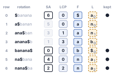
The stretch for ana holds rows 2 and 3. Row 2 is not marked. It ends in n1, so one LF step takes it to row \(C[\texttt{n}] + 1 = 6\), which is marked with position 2. So row 2 is position \(2 + 1 = 3\). Now do row 3 yourself.
Row 3 ends in b0, so one step takes it to row \(C[\texttt{b}] + 0 = 4\), marked with position 0: row 3 is position \(0 + 1 = 1\). Positions 3 and 1, as the suffix array said.
The index keeps these samples from the moment it is built. Its constructor reads them off the suffix array in one pass over the rows, before the suffix array is thrown away:
Leave out the rate and it is SAMPLE, 32.
Then locate(p) turns every row of _interval(p) into a position with _position_of, which walks by LF one step at a time. The whole of locate is in fm_index.py.
The rate is a dial between space and time. Sample more often, and the samples cost more space; sample less often, and every position costs a longer walk. Here is the library’s index on the ten books, at three rates:3
| one sample every | index size | time per position found |
|---|---|---|
| 16 positions | 0.882 \(n\) | 1.2 µs |
| 32 positions | 0.685 \(n\) | 2.4 µs |
| 64 positions | 0.586 \(n\) | 4.6 µs |
Sample half as often and the time doubles, as an average walk of half the rate predicts, while the size drops each time by only half as much as before. Only the samples shrink, and the compressed column underneath stays the same size.
3.8.2 Getting the words back
The text is gone. To show Leo his line, the index has to produce it, and it has nothing to produce it from but the walk. LF walks the text backwards, emitting the letter in L at every row. So to read a range, start at a known row after it and walk back.
Say the range starts at position \(s\) and is \(\ell\) characters long. Then it ends at \(e = s + \ell - 1\). A second list of samples, kept when the index was built (_isa_samples in the constructor’s loop), holds the row of every 32nd position. Let \(t\) be the first kept position greater than \(e\). Starting from \(t\)’s row, the walk takes \(t - s\) steps and gives the letters from position \(t - 1\) down to \(s\). Reverse them and keep the first \(\ell\); the ones past the range are dropped.
Take banana$ at a rate of 2, where positions 0, 2, 4 and 6 are kept, in rows 4, 6, 5 and 0, and extract \(s = 1\), \(\ell = 2\):
- The range ends at \(e = 1 + 2 - 1 = 2\), so \(t = 4\), kept in row 5.
- The walk takes \(t - s = 3\) steps, rows 5, 2 and 6, and emits
a,n,a: positions 3, 2 and 1. - Reversed, that is
ana. Keep the first 2,an, which is positions 1 and 2 ofbanana$. Theaat position 3 is past the range and dropped.
Extracting \(\ell\) characters takes about \(\ell\) steps, plus at most the sampling rate to get from the sample to the end of the range. The check to write for it is plain: for every start \(s\) and length \(\ell\), what comes out must equal the \(\ell\) letters of the text that start at \(s\). The book can be read back out of its index, every line of it, from anywhere.
If the range runs so close to the end that no kept position comes after it, the walk starts from the row of position 0. That row’s rotation starts at 0, so its last letter is the final $. The walk gives the $ first, then the text from its end backwards. The code for extract, with its tests, is in the companion library, in fm_index.py.
3.8.3 From a hit to the whole quote
One last step, and it is the one Leo cares about. A hit is a position. He wants the quote: the whole line, whichever piece of it he remembered.
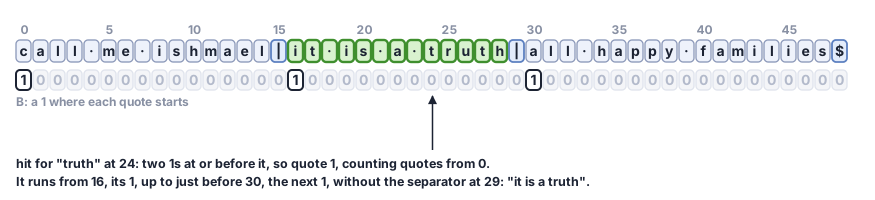
Make every quote a record, here a paragraph of a book, and join them all into one text, with a separator between neighbors and $ at the very end. Then keep one more row of bits, B, as long as the text, with a 1 wherever a record starts [25, Ch. 11]. Now a hit needs only counting, of the 1s in B. The number of 1s before position \(i\), not counting position \(i\) itself, is called rank, written \(\text{rank}(i)\). You met it in the search chapter, asked of a tree of keys: how many keys are smaller than this one. Here it is occ again, asked of a row of 0s and 1s, and checkpoints make it fast as they did for L.
Count the quotes from 0, as positions are counted: the quote that starts at position 0 is quote 0, and each 1 in B takes the number of the quote it starts. In the figure below, the hit for truth is at position 24. Count the 1s at or before position 24. There are two, so the hit is in quote 1. It runs from quote 1’s own 1, at 16, up to just before the next 1, at 30, and leaves out the separator at 29. The last quote has no next 1, so it runs up to just before the $ at the end. Extract what is between, and that is the quote. In numbers, for the hit at 24:
\[\text{quote} = \text{rank}(25) - 1 = 1,\qquad \text{start} = 16,\qquad \text{separator} = 30 - 1 = 29,\]
so the quote is positions 16 to 28, it is a truth. The count asks rank about 25, one past the hit, because rank leaves out its own position. With a checkpoint every 16 positions, \(\text{rank}(25) = \text{rank}(16) + 1 = 2\): the checkpoint at 16 holds the 1 at 0, and the bits from 16 to 24 hold one more, at 16.
Storing the answer for every position would cost a whole number per bit, far more than the bits themselves, and counting from the start every time is a scan. The way out sits between the two: the checkpoints from above, in two layers.
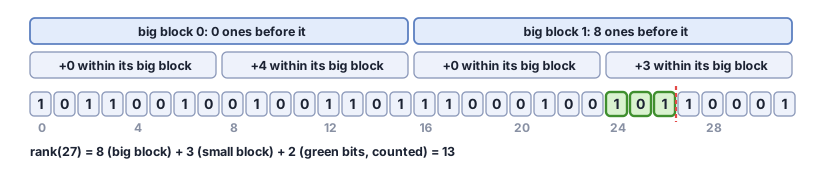
Cut the bits into small blocks, and the small blocks into big blocks. For every big block, store how many 1s come before it: a full-size number, but there are few big blocks. For every small block, store how many 1s come before it within its big block: many of those, but each one is small, because it can never exceed the size of a big block. Then \(\text{rank}(i)\) is the big block’s number, plus the small block’s number, plus a count of the few bits between the start of \(i\)’s small block and \(i\). Two lookups and a short count, however long the row of bits is [26]. With the sizes real systems use, the two tables together add only a small fraction of the size of the bits themselves.
Because the first record starts at position 0, every hit has a 1 at or before it, and so wherever a hit falls inside a quote, the count less one is that quote’s number.
Both steps are questions you have met. The count is \(\text{rank}(p + 1)\) for a hit at \(p\). Finding where a given 1 sits is rank’s partner, select: the search chapter’s other question, which key is in position \(j\), asked of bits. \(\text{select}(j)\) is the position of the 1 that starts quote \(j\), the one with \(j\) 1s before it, so on B \(\text{select}(0) = 0\) and \(\text{select}(1) = 16\). With both, for a hit at \(p\):
- quote \(= \text{rank}(p + 1) - 1\),
- start \(= \text{select}(\text{quote})\),
- separator \(= \text{select}(\text{quote} + 1) - 1\).
The hit is used exactly once, for one rank, and then forgotten. Everything after it depends only on which quote it fell in. So a fragment from the start of a quote, from the middle, or from the last three words costs the same. That is the property Leo needed, and it took nothing new: rank and select, two questions you have already met, asked of one more row of bits.
The separator can’t be another $, because the transform needs $ exactly once. So the separator is a second reserved byte, and both are kept out of the quotes. A record that holds either is refused with an error when the whole collection, the corpus, is built. A fragment that holds either finds nothing when it is asked. That second rule is what keeps a match from straddling two quotes. A fragment that crosses from the end of one quote into the start of the next would have to contain the separator, and no fragment may.
Any quote finder must get these cases right. Each one catches a slip that is easy to make, by hand or with an AI:
- A hit on the first byte of a quote returns that quote, not the one before it. The slip is counting only the 1s before the hit: the hit sits on its quote’s own 1, so the count comes out one short.
- A hit on the last byte of a quote returns that quote, without the separator after it. The slip is keeping the separator on the end of the quote.
- A hit in the last quote returns that quote whole, up to just before the
$. The slip is looking for a next 1 that is not there. - A fragment that runs from the end of one quote, across the separator, into the start of the next finds nothing. The slip is forgetting that rule, so a match runs from one quote into the next.
The library’s Corpus gets all four right. Here they are on the three quotes of Figure 3.19, one line each, in the order of the list:
from algodesign.strings import Corpus, SEPARATOR

corpus = Corpus([b"call me ishmael", b"it is a truth", b"all happy families"])
def quotes(fragment):
    return [q.text for q in corpus.find(fragment)]

print(quotes(b"it is"))     # [b'it is a truth']
print(quotes(b"truth"))     # [b'it is a truth']
print(quotes(b"families"))  # [b'all happy families']
crossing = b"ishmael" + bytes([SEPARATOR]) + b"it"
print(quotes(crossing))     # []
Now run it on the ten books, cut into 22,703 paragraphs. Type drizzly November, and back comes a paragraph of Moby-Dick, whole, 1,115 bytes of it: “Call me Ishmael. Some years ago…”, on through the drizzly November and on to the end of the paragraph, with the line breaks of the printed edition still in it. Type in my soul, and six paragraphs come back from four books: Shelley’s Frankenstein, three places in Moby-Dick, Great Expectations and Dracula. Type universally acknowledged, and both paragraphs from earlier come back, Austen’s opening and Dickens’s poet. Not one of those quotes was stored anywhere as text.
3.8.4 What it costs
The index the library ships, built over the ten books with one sample every 32 positions (the middle row of Table 3.5), takes 0.685 bytes for every byte of text: 4,656,156 bytes, against 6,793,687 bytes of text and $. It is smaller than the book, and the book is not kept. Against the text plus a suffix array, at \(5n\), it is 7.3 times smaller. In that space it counts, finds and quotes. On the library’s fast Rust build, counting an eight-letter fragment and finding each of its positions both take a few millionths of a second.4
How few bits the column needs depends on how predictable each letter is from the letters around it, which the compression chapter measures as the text’s entropy. The sorted order puts letters that keep the same company side by side, and the black box that holds the column is built to make use of that.
The 0.685 bytes are paid for in speed, since every count is decoded from the compressed column, and for Leo’s flood the space is the cost that decides. One index also has a size limit, so a large service cuts its corpus into pieces between quotes.
Compare the compressed index with a plain one, which keeps the column as bytes with a running count every 512 rows and stores the samples and marks uncompressed: about two bytes for every byte of text. Timed side by side in the same run as above, the compressed index is about 3 times slower to count and to read back, and about 6 times slower to locate, in return for a third of the space.5 Most of the locate gap comes from the compressed marks, read at every step of the walk, and the packed samples, not from the column.
One index cannot grow forever, though. The library stores its positions as 4-byte numbers, which reach about 4.29 billion characters, and building an index holds several arrays of \(n\) numbers in memory at once. Leo’s flood is far bigger than that. So a service cuts the collection into pieces of a few gigabytes, always between two quotes, builds an index for each piece, asks every piece the same question, and merges the answers. Because no cut falls inside a quote, every quote is found whole, in one piece.
The design holds up at sizes far past ten books. In 2025 a team built this same kind of index over 83 terabytes of web text, on raw bytes exactly as this chapter does, and the index came to 44% of the size of the text it replaced [27]. Because the index reads bytes, not letters, it works the same on text in any language.
The library states the invariant of backward search in the proof assistant Lean, in lean/AlgoDesign/Strings/FMIndex/Spec.lean, and proves it in FMIndex/Search.lean: a row lies in the stretch backward search returns exactly when the suffix in that row begins with the pattern, for any text that ends in a single $ and any pattern without $ before its end. A second theorem says the count it gives is the number of positions where the pattern occurs. For the records, a third says that the hit lies between the bounds two selects give for its record, the one its rank less one numbers. Two more say that a search returns exactly the records containing the fragment, each once and in order, and that each comes back whole.
The proofs are about texts written as lists of numbers, with the last column counted plainly and rank and select read straight off the row of bits, not through the directory. The compressed column, the black box above, has no proof of its own; it is held to the plain version by tests. And no proof says anything about whether exact bytes was the right thing to search for, which is the question the curly apostrophe asked earlier in the chapter.
3.8.5 What a frozen index can’t do
Every structure after the Patricia tree was built once and then only asked questions. The FM-index is the extreme case: it is a single sorted arrangement of the whole text, and one new quote, added anywhere, changes rows all through it. To add a book, you build the index again. For a library of Gutenberg classics that is fine; nobody is adding chapters to Moby-Dick. For a corpus that grows every day, it is the assumption that breaks, and the practice section comes back to it.
3.9 ✎ When the ground shifts practice
A service has 100 GB of text that never changes, and it must answer millions of “where does this fragment occur?” questions a day from a machine with 128 GB of memory. A colleague proposes a suffix array, “because it’s the standard”. Say what that proposal would need in memory, and which structure in this chapter fits instead. Then say which of the three questions, count, locate and extract, gets slower in exchange, and which setting decides by how much.
The same service now receives about a thousand new documents every day, and they must be searchable within the hour. Name the assumption the FM-index was built on that this breaks. Then describe a design that keeps most of the index’s advantages anyway, without rebuilding the whole thing every hour. (A hint: the search chapter’s LSM-tree stopped repairing and started stacking.)
A hospital stores the genomes of ten thousand patients, each about three billion letters, and each differs from the others in only about one letter in a thousand. Someone builds this chapter’s FM-index over one genome, multiplies its size by ten thousand, and gets about the right size for an FM-index of the whole collection. Say why that is still far more than the collection really holds, which property of this collection the FM-index ignores, and what a better measure of its size would count. Think about the runs in the transform.
3.10 ◆ What these are actually made of big picture
This chapter built nine structures, from a plain scan to an index that replaces its book. That sounds like nine things to remember. Open them up, and they are made of a handful of small ideas, several of which you met in the search chapter doing completely different jobs.
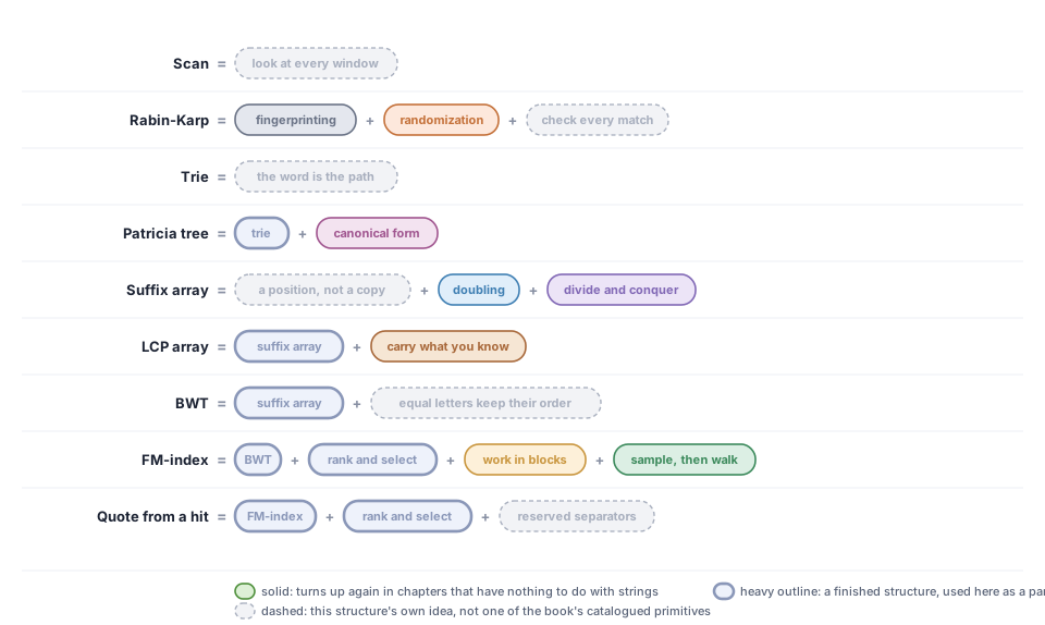
Scan = look at every window. No preparation, no invariants, and every question re-reads everything. Every other structure here is an attempt not to.
Rabin–Karp = fingerprinting + randomization + check every match. Fingerprinting: compare two small numbers instead of two long strings, and accept that equal numbers only mean maybe. Randomization: pick the modulus at random, so nobody can write a text that fools it every time. Check every match: a maybe is confirmed against the real characters before it is reported, which is what makes the method exact. The Bloom filter in the search chapter made the opposite choice: it never checks, and accepts being wrong in one direction.
Trie = the word is the path. Nothing stores a word; the words are the routes down the tree, and shared beginnings are walked once.
Patricia tree = trie + canonical form. Every node below the root branches or ends a word, and every insert and removal restores that invariant before it finishes, so each set of words has one standard shape, its canonical form. That invariant is what keeps the tree at most two nodes per word, whatever the words look like.
Suffix array = a position, not a copy + doubling + divide and conquer. Store where each suffix starts, never its letters. Sort by doubling, so two numbers from the last round stand in for twice as many letters. Then search by divide and conquer, halving the range, exactly as binary search did in the search chapter.
LCP array = suffix array + carry what you know. The count of matching letters is carried from one position to the next (carry what you know), because it drops by at most one (the appendix shows why), so no letter is compared from scratch twice.
Burrows–Wheeler transform = suffix array + equal letters keep their order. Read the letter before every sorted suffix, and the text becomes a permutation of itself that can be walked backwards. The transform is the one idea here that belongs to strings alone, and the compression chapter uses it again for a different end.
FM-index = BWT + rank and select + work in blocks + sample, then walk. Backward search turns every question into counts of a letter above a row, and each of those counts is one rank. Checkpoints kept in blocks (work in blocks) make rank fast in little space, as fat nodes made the B-tree fast on disk. Sample, then walk keeps only every 32nd position and recovers the rest by walking, which is a dial between space and time that you set.
Quote from a hit = FM-index + rank and select again + reserved separators. One rank finds the quote, two selects bound it. The same two questions, asked of one more row of bits.
3.10.1 Choosing one, under pressure
Every structure here makes a promise. Break what the promise needs and the answers are wrong. Break what makes it a good choice, and the answers are still right, but you are paying for the wrong thing. Each row is a short contract, in the contracts chapter’s sense. The last column is its failure mode: what you see when what the promise needs is broken. In every row, unless something guards against it, you see no error at all, just a wrong answer.
| structure | the promise needs | it is a good choice when | if it breaks |
|---|---|---|---|
| Scan (Rabin–Karp) | every fingerprint match is checked against the text | the text is searched once, or changes all the time, because every question re-reads all of it | a false alarm is reported as a match, at a position where the pattern is not |
| Trie, Patricia tree | the stored keys, and nothing else, end at marked nodes | the fragment and a key must agree from their first letter, as in autocomplete or a router’s table | a removed word that keeps its mark is still found, and autocomplete goes on offering it |
| Suffix array | the array is the sorted order of the suffixes of this text | any fragment must be found, the text rarely changes, and it fits several times over in memory | after the text changes, the search returns positions where the fragment no longer is, and misses where it now is |
| FM-index | the text ends in one unique $, and the index was built from it |
the text is large, fixed and searched often, space matters more than a few microseconds, and a position is answer enough | the rotations stop sorting like the suffixes, and a fragment is found running off the end of the text and around to its start; after the text changes, positions point at the wrong places |
| Quote from a hit | no record holds a reserved byte, and no fragment does either | answers must be whole records, whichever piece of one was remembered | a match straddles two quotes, and back comes a quote that does not contain the fragment |
3.10.2 What each one costs
For a text of \(n\) characters, a fragment of \(m\), and \(z\) occurrences of it. Sizes include everything that must be kept to answer, the text too when it is needed.
| structure | prepare | count | locate | size |
|---|---|---|---|---|
| Scan (Rabin–Karp) | nothing | about \(n + m\) steps, expected, plus \(m\) per occurrence | the same | the text, \(n\) |
| Patricia tree, of \(k\) keys | about the total length of the keys | \(m\) steps, plus a step per answer | the same | at most \(2k\) nodes, plus the keys |
| Suffix array | about \(n \log_2 n\) steps by doubling | about \(2m \log_2 n\) comparisons | plus \(z\) | \(5n\) bytes, text included |
| FM-index | the suffix array, once | \(2m\) counts | plus at most the sampling rate in steps per occurrence | 0.685 \(n\) on the ten books, with one sample every 32 positions, text not needed |
Three things the table says that its cells don’t.
Only one row doesn’t need the text. Every other structure keeps the book and adds to it. The FM-index is the book, in a form that also answers questions.
The FM-index’s count takes the same number of steps for any \(n\). Two counts per letter of the fragment, whether the text is banana$ or a library. What grows with the text is the number of occurrences to find. Each costs at most the sampling rate in steps, which you can trade for space with one setting.
The scan is still the right answer sometimes. For a text searched once, any preparation is wasted. For a text that changes every second, every index is out of date before it is built. A row nobody would choose for Leo is the right row for a log file being written as you watch it.
3.10.3 Where they run
Each of these runs inside programs in daily use.
| structure | where it runs |
|---|---|
| Rolling fingerprint | the substring search of Go’s standard library, as a fallback when plain comparison keeps failing, with a fixed base and every match checked, so it gives up the random prime the design assumes; file synchronization that sends only the parts of a file that changed, as rsync does; backup tools that cut files into pieces wherever the fingerprint of the last few bytes hits a chosen value, so inserting a few bytes changes only the pieces around the edit |
| Trie and Patricia tree | routers choosing where to send a packet (the router appendix); web servers matching a request’s path to the code that answers it; the indexes of some databases |
| Suffix array | finding text that repeats across a huge collection, such as the training text of a language model; building the transform |
| Burrows–Wheeler transform | compressors, bzip2 among them |
| FM-index | read aligners such as BWA [28] and Bowtie [29], which place short pieces of DNA on a reference genome |
One kind of program is missing from the table. A web search engine, or the search box of a mail program, keeps an inverted index, the machine-built index of words from the start of the chapter. Text in those programs splits into words, and an index of words is smaller and simpler. The structures here take over where text has no words to cut it into: a genome, a model’s training text, a file being synchronized, an address. Where any piece can be the question, an index of short pieces of text, the kind GitHub built for its code search, still serves, as a filter with a check behind it. Suffix indexes give exact counts and positions directly, and suit text prepared once and searched often.
3.10.4 The same ideas, over and over
| primitive | where else it turns up |
|---|---|
| fingerprinting | checking that two files match, the Bloom filter |
| randomization | quicksort’s pivot, hash tables, the treap |
| canonical form | sorting a list before removing duplicates, fractions in lowest terms |
| doubling | a growable array, galloping search, jumping up a tree by powers of two |
| divide and conquer | binary search, mergesort |
| carry what you know | a running total, sliding-window maximums |
| work in blocks | B-tree nodes, disk pages, cache lines |
| sample, then walk | checkpoints in a video file, the index of a long log |
Rank and select, the two questions under the FM-index, turn up as widely: in the search chapter’s ordered dictionaries, in compressed graphs, and in tree layouts stored as bits.
Most of these ideas came into this chapter from somewhere else, and every one of them leaves it for somewhere else again. When a problem arrives that no structure here fits, the useful question is which of these ideas it needs: what must be checked, what can be carried, what can be counted in blocks, and what you can afford to forget and recover by walking.
3.11 ◆ Where that leaves the quote big picture
Back at the dinner table. Somebody is talking about a long winter, and Leo has a fragment: “in my soul”. In the time it takes to put down his glass, an index smaller than the books it came from has found six paragraphs in four of them, and handed back, whole, the one he wanted. He says it, the table goes quiet for a second in the good way, and the conversation moves on carrying one more shared thing.
None of that needed a new idea at the moment it happened. Every piece of it was decided long before, by asking the same few questions of each structure in turn. What does the person actually remember: a start, a middle, any piece? What happens at question time, and what can be done once in advance? What has to be kept, and what can be thrown away and rebuilt by walking? And what does exact mean? As the curly apostrophe showed, that was a decision before it was ever an algorithm. The structures in this chapter are answers to those questions under one set of conditions. Change the conditions, and the same questions pick a different structure.
Almost everything this chapter named is what the rest of the world calls it too: pattern, window, fingerprint, trie, Patricia tree, suffix, suffix array, LCP array, Burrows–Wheeler transform, LF mapping, rank, select, FM-index, sampling. The table of longest borders, the prefix function, is also called the failure function. Open any implementation, read any paper, ask any model, and those words will be waiting.
A few were this chapter’s own. A false alarm is what the literature calls a spurious hit. To squeeze the chains is path compression, in tries; union–find uses the same words for something else. And Leo’s flood was only ever a name for a large corpus. They were scaffolding, and the ideas underneath keep their standard names.
The quotes were never really the point. Knowing what it costs to find any piece of a text, and what you can afford to keep, was.
3.12 ✎ Take a turn with the quotes practice
Two kinds of work follow. First, projects: you build something, measure something, or explain something to another person. They have no single right answer, so nobody can mark them for you. After them comes a bank of numbered exercises, each with one right answer you can check. The bank names the ones that use the appendix Why the fast versions are right. Do some of each: the exercises show what you know, the projects show what you can do. Where a project needs code, let an AI write it; the times given assume it does. Your part is what stays yours even when the AI helps: saying what the code must do, building the check that shows it does, and judging what comes back.
Project 1 · the FM-index · hard · ~2 hours
Build Leo’s quote finder. Download a handful of books from Project Gutenberg, from at least three continents and in at least two languages, one of them your own. Cut them into paragraphs, and have an AI build a quote finder over them that returns whole paragraphs for any fragment. Before you ask, write down your checks:
- for a thousand fragments cut at random out of the books, the finder returns every paragraph that a plain scan finds, and no other;
- a fragment that appears in no book returns nothing;
- the empty fragment returns every paragraph;
- a fragment that crosses the end of one paragraph into the start of the next is never reported as found inside either.
Build the checks yourself, and run them before you believe a single answer. Then count how many different bytes your books use, and say why it is more than the 126 of the ten books.
Project 2 · tries · ~45 min
Count the chains. Collect the opening sentences of a hundred novels you can find online. Have an AI store them in a trie and in a Patricia tree and report the node count of each. Before you run it, predict the ratio between the two counts, and say why. Then store the last sentences of the same hundred novels and compare. Explain the difference in words a friend who has not read this chapter would follow.
Project 3 · what is a character · ~1 hour
Decide what “exact” means. Take the corpus from Project 1 and add a step before indexing that rewrites every curly apostrophe and quotation mark as a straight one and every run of spaces and line breaks as a single space. Mind that a letter like č, stored as one character, is two bytes, so a search for c does not find it. Write down first, as a specification, exactly which differences your finder now ignores and which it still respects. Then find a fragment that the normalized finder matches and the raw one doesn’t, and one where normalizing makes the answer wrong by your own specification. If you can’t find the second, say why your specification rules it out.
Project 4 · the suffix array · hard · ~1.5 hours
Skip the letters you already know. The suffix-array search compares the pattern from its first letter on every look. Since the rows are sorted, a look between two rows that both share the first \(k\) letters with the pattern can start comparing at letter \(k\). To never compare a letter twice, the search also needs a table, worked out once from the LCP array: for every pair of rows it can land between, how many letters their suffixes share. Have an AI write that faster search, with its table. Specify the check first: it returns exactly what the plain search returns, on every fragment you try, including the empty one and one that occurs nowhere. Then measure both on a whole book, with fragments of length 5, 20 and 100, and say whether the saving pays for the extra table.
Project 5 · the LCP array · ~45 min
Find what a book repeats. Pick a book, have an AI compute its suffix array and LCP array, and list the ten longest passages that occur at least twice. Before you look, guess what they will be. Then explain each one: a refrain, a chapter heading, a phrase a person in the book keeps saying, a printing convention. Which of them would a reader call a repetition, and which only a machine would?
Project 6 · the FM-index · ~1 hour
Turn the dial. Build the quote finder from Project 1 with one sample every 4, 16, 64 and 256 positions. For each, measure the size of the index and the time to locate every occurrence of a common word. Plot both against the rate, and say which rate you would ship for a phone, for a laptop, and for a server that answers a million questions a day, and why the three answers differ.
Project 7 · the quote finder · hard · ~2 hours
Visit each quote once. The quote finder locates every hit and then keeps each quote once, so a common word that occurs ten thousand times inside forty quotes costs ten thousand walks to return forty answers. Have an AI build a finder whose cost grows with the number of quotes it returns, not with the number of hits, and have it explain the extra structure that needs and what it costs in space. Specify the check first: on every fragment you try, it returns exactly the quotes the plain finder returns. Then measure both on fragments that occur ten, a thousand and a hundred thousand times, and say where the extra structure pays for itself.
Project 8 · design · hard · ~2 hours
Keep a changing library searchable. New books arrive every day, and a book already stored can be corrected or taken down. Every search must return each paragraph that holds the fragment now, exactly once: never a paragraph from a book that was taken down, never the old wording of a corrected one, never the same paragraph twice. No structure in this chapter does that alone. Design an arrangement that does, and write it as a design box of your own: a goal, an idea, and the invariants it keeps. Say how its pieces work together on one search. Then build the smallest example that catches a design breaking one of your invariants: a few books, one correction, one removal, one fragment. Have an AI build the arrangement, and run your example before you believe it.
Project 9 · the suffix tree · ~1 hour
Measure why the tree doesn’t fit. By hand, put every suffix of banana$ into a trie, then squeeze its chains as the Patricia tree does. Count the nodes of each, and find ana in both. Then have an AI insert every suffix of the first 1,000, 2,000 and 4,000 characters of a book into a trie and into a Patricia tree, and report the node counts. Check your counts against the growth the chapter states. Then estimate the bytes per character of text for each, if every node takes about 24 bytes.
A quote finder joins its paragraphs into one text before indexing them. To keep things simple, the person who wrote it joined them with a single space instead of a reserved byte, and every test they wrote passed. Here is the part that joins:
text = b" ".join(paragraphs) + ENDEND is the end marker, the chapter’s $.
- Before running anything, say what kind of fragment this version gets wrong, and what wrong answer it gives. The section From a hit to the whole quote has the reason.
- Write the smallest input that shows it: two paragraphs and one fragment. Smallest means fewest characters. If yours has more than twenty, keep cutting.
- Now take the first two paragraphs of Pride and Prejudice, which end and begin “…in want of a wife.” and “However little known…”, and say what this finder returns for the fragment
wife. However. Then say what it should return.
Only after you have your own answer: hand the line to an AI and ask what is wrong with it. Does its answer find the problem? A space looks like a perfectly good separator in one line of code. Whether it is depends on a rule that lives in another part of the program, which the AI was not shown.
3.13 ✎ A bank you can mark yourself practice
Here are forty exercises. Each shows roughly how long it takes, and everything you need for them is in the chapter so far or in its appendix Why the fast versions are right. You can mark much of it by running the library on the same input: an array, a column, a count, the positions found or the quote returned. The steps on the way, such as each window’s fingerprint or a count of comparisons, you check by hand against the chapter. The answers are on a page of their own.
If you only do four, do Exercises 4, 10, 19 and 24.
They are grouped by kind of task, not by structure. To practice one structure, here are the exercises for each section:
- Reading the whole book, every time: 1, 2, 20, 21, 22, 26, 27
- I remember how it starts: 3, 4, 19, 23, 28, 37, 38, 40
- It was somewhere in the middle: 5, 6, 7, 15, 16, 18, 24, 29, 30, 31
- Useful mess?: 8, 9, 17
- By heart: 10, 32, 33
- Give me the whole line: 11, 12, 13, 14, 25, 34, 35, 36, 39
One uses the chapter’s appendix: Exercise 6 needs its part on Kasai’s method.
3.13.1 Run it and report the state
Exercise 1 · gentle · ~5 min
Slide the pattern aab along the text aabaacaabaab by hand, comparing character by character and moving on at the first mismatch. Where does it occur, and how many character comparisons did the whole scan make?
Exercise 2 · middling · ~15 min
The text is the digits 6404137153929 and the pattern is 153, base 10, modulus 13. Write down the fingerprint of every window of three digits, rolling each from the one before. At which positions do the fingerprints agree with the pattern’s, and which of those are false alarms?
Exercise 3 · gentle · ~10 min
Insert tea, ten, to, inn, in, tent into an empty trie, in that order. How many nodes does it have, root included? How many after squeezing it into a Patricia tree? What does keys_with_prefix("te") return, in order?
Exercise 4 · middling · ~15 min
Insert romane, romanus, romulus, rubens, ruber into an empty Patricia tree and draw it, every branch labelled. Then insert rubicon. Which branch is cut, and where? How many nodes does the tree have before and after?
Exercise 5 · gentle · ~15 min
Write the suffix array of abracadabra$, with $ sorting before every letter. Which rows hold the suffixes that begin with abra, and which text positions are they?
Exercise 6 · middling · ~20 min
From the suffix array of abracadabra$ (the previous exercise), write its LCP array. What is the longest passage that occurs twice, and which entry tells you? Then fill it in Kasai’s way: visit the positions in text order, 0 to 11, carrying h. For each position, what does h start at, and what does it record?
Exercise 7 · middling · ~20 min
Sort the suffixes of aababa$ by prefix doubling. Give the tag of every position after each round, with tags starting at 1 and $ tagged lowest, until every tag is different. How many doubling rounds did it take, not counting round 0, the tagging by single letters?
Exercise 8 · gentle · ~15 min
Write the Burrows–Wheeler transform of abracadabra$: sort its rotations and read the last column. Where are the runs of equal letters?
Exercise 9 · middling · ~15 min
A last column reads omotta$. Recover the text with the LF walk: sort the column to get F, number equal letters, start from the row whose last letter is $, and follow LF. Give the LF value of every row, and the text.
Exercise 10 · middling · ~15 min
Using only the last column of abracadabra$ (Exercise 8) and its table C, run backward search for bra. Give the interval of rows after each letter, and the count.
Exercise 11 · gentle · ~10 min
For the bits 0110100111000101 (position 0 first), what are rank(5), rank(11) and rank(16), the number of 1s before each position, and select(0), select(4) and select(7), counting the 1s from zero?
Exercise 12 · middling · ~20 min
The FM-index of abracadabra$ keeps a sample at every 4th text position (0, 4 and 8). Find every row whose suffix begins with a, and turn each into its text position by walking LF to a sampled row. How many steps does the longest walk take?
Exercise 13 · middling · ~15 min
The FM-index of abracadabra$ keeps the row of every 4th text position (0, 4 and 8). Extract the 3 letters starting at position 5, then the 2 letters starting at position 9. For each: which row do you start from, how many LF steps do you walk, and what comes out?
Exercise 14 · gentle · ~10 min
Three quotes are joined into one text with a separator between them: frankly my dear, here is looking at you, may the force be with you. The fragment looking is found at one position. Which position, which quote does it fall in, numbered from 0, and which bounds do the two selects give? Then: which quotes does a search for you return?
3.13.2 Which promise broke
Each item hands you something a program produced and claims is correct. Say whether it is, and if it is not, name the invariant it breaks and the smallest change that would mend it. One of them is correct, and saying so is the answer.
Exercise 15 · middling · ~10 min
The suffix array of cocoa$ is 5 4 0 2 3 1.
Exercise 16 · middling · ~10 min
The suffix array of pepper$ is 6 1 4 0 3 2 5.
Exercise 17 · middling · ~10 min
A last column reads ap$p$le, and is said to be the transform of some text.
Exercise 18 · middling · ~10 min
The LCP array of cocoa$ is 0 0 0 3 0 1.
Exercise 19 · middling · ~10 min
A Patricia tree holds cart and card. Below the root it has a branch labelled ca to a node that holds no word, from there a branch r to a node that holds no word, and from there two branches, t and d, each ending a word.
Exercise 20 · middling · ~10 min
A fingerprint search for 15 in the digits 31415926, base 10, modulus 7, reports the positions [3, 5].
3.13.3 You supply the input
Exercise 21 · middling · ~15 min
Find a text of 10 letters and a pattern of 4, both over the letters a and b, that make the plain scan do as many character comparisons as it possibly can. How many is that?
Then: Say what every text and pattern that reach the maximum have in common.
Exercise 22 · gentle · ~10 min
With base 10 and modulus 13, find two different three-digit windows that have the same fingerprint.
Then: Say the rule that decides, for any two numbers, whether they get the same fingerprint.
Exercise 23 · gentle · ~10 min
Choose five words of four letters each so that the trie holding them has as many nodes as possible. How many is that, and how many nodes does the Patricia tree of the same words have?
Then: What does that say about when squeezing pays most?
Exercise 24 · middling · ~15 min
Choose a text of 8 letters over a and b, with $ added at the end, that makes prefix doubling run as many rounds as possible. How many doubling rounds does it take, not counting round 0, the tagging by single letters?
Then: Say which property of the text decides the number of rounds.
Exercise 25 · middling · ~10 min
A quote finder joins its quotes with a reserved separator, written | here, and refuses any quote that holds it. It does not check the fragment it is asked for. With the quotes you had me at hello and show me the money, write a fragment that this finder reports as found, though neither quote contains it.
Then: Say why keeping the separator out of the quotes is not enough on its own.
3.13.4 Which idea do you reach for
Each of these nine exercises describes a situation, most of them far from quotes, and asks which of the ideas above, the eight primitives or rank and select, you would use. Each has four options: pick the one you would reach for first.
Exercise 26 · gentle · ~5 min
A multiplayer game must check, sixty times a second, that every player’s copy of the game world is still the same as the server’s. Sending the whole world each time is far too slow, and a very small chance of missing a difference is acceptable.
- fingerprinting
- divide and conquer
- sample, then walk
- work in blocks
Exercise 27 · middling · ~5 min
A public web service checks whether a pasted paragraph appears in its archive using a rolling fingerprint with a fixed, published modulus. An attacker sends texts that make every window match, and the service slows to a crawl.
- carry what you know
- randomization
- rank and select
- canonical form
Exercise 28 · middling · ~10 min
A phone keyboard suggests words while you type. The team wants the stored dictionary compact, and still to be correct after words are added and removed every day.
- doubling
- canonical form
- fingerprinting
- sample, then walk
Exercise 29 · middling · ~10 min
You must sort the positions of every line break in a ten-gigabyte log by what follows them, and many lines repeat long stretches word for word, so comparing strings directly keeps re-reading the same letters.
- doubling
- randomization
- work in blocks
- rank and select
Exercise 30 · gentle · ~5 min
A sorted list of every street name in a country is printed in a thick book, with no index. You need the page where names starting with Mill begin.
- carry what you know
- sample, then walk
- divide and conquer
- fingerprinting
Exercise 31 · hard · ~15 min
The suffixes of a long text are sorted, one to a row. For every row you need how many opening letters its suffix shares with the suffix in the row above, and computing each one from scratch is far too slow.
- carry what you know
- work in blocks
- randomization
- canonical form
Exercise 32 · middling · ~10 min
A map app stores, for a billion road segments, one bit saying whether each is a toll road. It must answer how many toll segments come before segment i instantly, and may use only a little more memory than the bits.
- fingerprinting
- rank and select
- divide and conquer
- doubling
Exercise 33 · middling · ~10 min
Storing a running count after every bit of that billion would cost far more than the bits; counting from the start on every question is far too slow. Each question may read only two stored counts and one machine word of bits.
- sample, then walk
- work in blocks
- randomization
- carry what you know
Exercise 34 · middling · ~10 min
A bank numbers every transaction on an account since it was opened, ten years of them, and must quickly show the balance after any numbered transaction, without storing a balance after every transaction.
- divide and conquer
- canonical form
- sample, then walk
- rank and select
3.13.5 The tests pass. What did they miss?
Code that fails its tests is easy to catch. The costly kind passes every test, because nobody wrote a test for the requirement it breaks.
Exercise 35 · middling · ~15 min
A team ships a quote finder built on an FM-index. Its tests pass: for a thousand random fragments, count agrees with a plain scan of the books, and locate returns exactly the positions the scan finds. In production, people type quotes with straight apostrophes copied from a chat, and the finder says they appear nowhere. What requirement did the tests miss?
Then: Write the requirement as a sentence a test could check.
Exercise 36 · hard · ~20 min
An index over song lyrics returns whole songs for a fragment, joining the songs with a reserved separator. Its tests pass: every fragment cut from inside one song returns that song and every other song containing it, and a fragment that occurs nowhere returns nothing. After launch, a lyric site adds one song containing the separator byte inside a line, and from then on some searches return songs that do not contain the fragment. What requirement did the tests miss?
Then: Say where the checks belong, and what each must do.
3.13.6 Fix the code, the box, or the design?
Each item starts from code an AI wrote from one of the chapter’s design boxes, and something it did that looks wrong. Decide which of three things happened. The code breaks a promise in the box: fix the code. The code keeps the box but misses what you wanted: fix the box. The design keeps its promise, but its assumptions or its cost no longer fit the job: change the design. Say why.
Exercise 37 · middling · ~10 min
You give an AI the trie’s design box and ask for the code. Its remove walks to the word and clears the mark that says a word ends there, and nothing else. Insert tea and ten into an empty trie, then remove both. get finds neither word, keys() returns nothing, and the count of words is 0. The trie still has 5 nodes. Which of the three is it, and why?
Then: Suppose the box had stopped at invariant 2 and said nothing about memory. Which would it be then? Write the line you would add to the box, and a test you would keep from the AI that checks it.
Exercise 38 · middling · ~10 min
The same AI’s trie, its remove now mended, holds 2,000 web addresses of a shop, such as https://shop.example.com/products/aaliwuqonsmb/reviews, about 54 letters each. Nothing has been removed, every check of the box’s invariants passes, and every lookup is right. Yet the trie has 36,601 nodes, about 18 per address, and a colleague says the leak is back. Which of the three is it, and why?
Then: Name the design you would switch to, and say what you would measure to check it.
Exercise 39 · middling · ~10 min
An AI builds the FM-index from its design boxes for a reading app. Asked where i occurs in mississippi$, locate returns [10, 7, 4, 1]; asked for ssi, [5, 2]. The app jumps to the first position in the list, so a search for i takes the reader to position 10, the last i in the text. Which of the three is it, and why?
Then: Rewrite the line of the box that has to change, say what the change costs, and name a test you would keep from the AI.
3.13.7 Taking a word out of a squeezed tree
Exercise 40 · hardest in the chapter · ~90 min
You already have:
- the Patricia tree’s
insert, printed in the chapter - its invariant: every node below the root branches or ends a word
- the chapter’s one-paragraph description of removal
Write remove(key) for the Patricia tree, as code or as precise steps, so that the invariant holds again after every removal. Your answer must say what happens to a node left with no word and no children, to one left with a single child and no word, and why the root is treated differently from every other node.
Three checks tell you whether you got it right, on the words romane, romanus, romulus, rubens, ruber, rubicon, rubicundus, removing romulus, then rubicon, then rubicundus:
- After every removal, no node below the root has exactly one child and no word.
- The tree after removing a word has exactly as many nodes as a tree built from scratch from the words that remain.
- Removing a word that is not stored changes nothing.
Stretch: The second check says a squeezed tree depends only on its set of words, not on the order they arrived in or were removed. Prove it.
Put this somewhere you’ll see it in about a week, and when you do, answer from memory first: no scrolling back, and no AI. Getting it wrong and then looking is the point; looking first isn’t.
- Name the structures in this chapter in order, and for each, the thing about Leo’s question it could not handle, which forced the next one.
- Why does a fingerprint match have to be checked against the actual characters, and what does the check cost when the fingerprints almost never agree by accident?
- What invariant does a Patricia tree keep about every node below its root, and why does it keep the tree small?
- Write the suffix array of
abab$by hand, and findabin it. - The transform of a text is exactly as long as the text. So where does the FM-index’s saving come from?
- A colleague’s FM-index answers every count correctly, but locate takes a full second per occurrence on a large corpus. What did they most likely set, and what does changing it cost?
Whichever of those you couldn’t reconstruct is the one to reread, and only that one. If you got all six, come back again in a month instead.
3.14 ★ Frontier map advanced
What follows is optional: a short tour of ideas just past the edge of this chapter, not the next step in its sequence. Skip it now if you’d rather move on, and come back later.
One thread runs through all of it. This chapter took a text as a fixed row of bytes, asked for exact matches, and built an index once. Almost every piece of current research changes one of those choices: what the pieces of a text are, whether it is one line at all, what counts as a match, or whether the text stays still. The rest asks what impossible really means. Each entry below names one of them, and most end with a question you can now ask of any system that makes it.
3.14.1 Did the AI copy this?
Exact indexes over training data
Language models are trained on trillions of words of text, and they sometimes give some of it back word for word. Finding out when is exactly Leo’s problem, at a scale no scan can touch: given a paragraph the model wrote, does it occur in the training text, and where?
The structures of this chapter are what the field reaches for. A 2022 study built a suffix array over a large training corpus and found that one 61-word sentence occurred more than 60,000 times in it. Removing such repeats before training cut how often the model reproduced its training text word for word to about a tenth [30]. A suffix array over five trillion tokens now counts any phrase in milliseconds [20], and in 2025 came an FM-index over 83 terabytes of web text, built on raw bytes and smaller than the text [27]. The same team uses it to find benchmark questions that leaked into training text, and a related tool traces a chatbot’s answer back to the exact training documents it echoes, in seconds [31]. That last one is this chapter’s from a hit to the whole quote, in a public tool, in 2025.
The FM-index among them makes the choice this chapter made about the apostrophe: it indexes bytes, not the model’s own pieces of words, so the index still works when the model, or the way it cuts text into pieces, changes.
The question to ask: an AI says its answer is original. What would you index, at what unit, and what would your check still miss: a paraphrase, a translation, a quote with one word changed?
3.14.2 A thousand copies of almost the same book
Repetitive collections and dynamic indexes
Every version of Wikipedia. Every release of a code base. The genomes of ten thousand people, each differing from the others in about one letter in a thousand. These collections are enormous, and almost all repetition. An FM-index measures its size against the text’s length, and that is the wrong measure here: ten thousand near-copies are not ten thousand times harder to index than one.
The transform already points to the fix. Near-copies make the last column fall into long runs of equal letters, and the number of runs, not the length, measures what is really there. A 2020 result showed how closely that count of runs tracks other measures of repetition [32], and the r-index answers count and locate in space proportional to the number of runs, not to the length [33]. Choosing which measure of repetition is the right one is a question of compression, and the compression chapter takes it up.
The other assumption this chapter made, that the text never changes, is falling too. Since 2022 a suffix array can be kept up to date through insertions and deletions, each in time that grows only like a power of \(\log n\), without a rebuild [34]. In 2026 a compressed index for repetitive text beat earlier updatable ones by up to 77 times on updates and up to 11 times on locating, measured on 37 GB of Wikipedia and 59 GB of human chromosomes [35]. Updatable indexes still trade something away, and when changes arrive in large batches, rebuilding from time to time can still be the better engineering.
The question to ask: your corpus is every version of one document. What should size mean for its index, and what does an update cost?
3.14.3 Placing a million reads
Minimizers
A DNA sequencer produces hundreds of millions of short reads, and each one has to be placed on a genome. Many current read mappers, especially for long reads, start with fingerprints. In every short stretch of a read they keep only the window whose fingerprint is smallest, its minimizer [36]. Two sequences that share a long enough stretch are guaranteed to keep the same minimizer inside it, so a handful of kept windows is enough to propose where a read belongs, and a careful alignment then checks the proposal [37]. It is the bargain from the start of this chapter again: a cheap fingerprint to guess, a real comparison to confirm.
The question to ask: which windows does your method keep, and what does it miss when two sequences share no kept window?
3.14.4 When there is no single text
Wheeler graphs
From about 2009, the most important text an FM-index searched was a human genome: a reference sequence of about three billion letters. A sequencer’s hundreds of millions of short reads are placed against it, many of them starting from exact matches that backward search finds, then aligned allowing differences. But no person’s genome is the reference. Everyone differs from it in millions of places, and a read from a part where you differ may align badly, or in the wrong place. So in 2023 a consortium published a first pangenome reference, built from the genomes of 47 people [38]. It is not one string. Where those people agree, it is a single path of letters; where they differ, it splits into alternatives and joins again. It is a graph.
Look again at why backward search worked. Every row was a position in the text, and the rows were sorted so that two things held. Rows were grouped by the letter that leads into them, which is what C relied on. And among rows that end in the same letter, LF kept their order: if row \(u\) came before row \(u'\), then \(\text{LF}(u)\) came before \(\text{LF}(u')\). It is the same rule: \(a_k\) in L is \(a_k\) in F. A text is a single path, and that path is what guaranteed such an order exists.
So ask for exactly that order on a graph. Put the nodes of a graph, whose edges carry letters, in one line so that:
- nodes with no edge coming in come first, and the rest are grouped by the letter on the edges coming into them, in alphabetical order;
- for two edges carrying the same letter, from \(u\) to \(v\) and from \(u'\) to \(v'\), if \(u\) comes before \(u'\), then \(v\) comes no later than \(v'\).
A graph that has such an order is a Wheeler graph [39], and on a Wheeler graph, backward search runs much as it does on a text: a stretch of nodes, narrowed one letter at a time by counting.
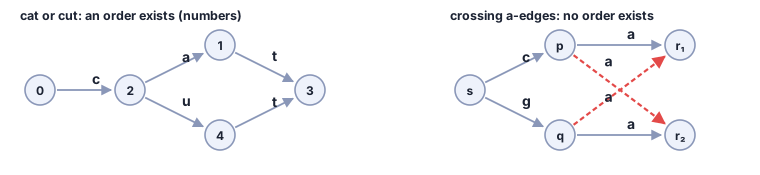
Not every graph has such an order, and the right-hand graph above shows why. The trouble is equal letters that cross: two a-edges whose starting points come in one order and whose ending points are forced into the other.
And here the field meets a wall. Deciding whether a graph has a Wheeler order at all is NP-complete as soon as its edges carry two different letters; with one letter it is quick [40]. The exact method in the same paper takes time that grows exponentially with the number of edges. Worse, for general graphs the whole idea of a fast search may be out of reach. Exact pattern matching in a graph cannot be done much faster than the size of the graph times the length of the pattern, unless a widely believed conjecture about the limits of computation, the Strong Exponential Time Hypothesis, is false [41]. A single line of text gets an index that answers in steps proportional to the pattern. A graph, in general, does not [42].
That is the shape of the problem genome researchers live with now: build graphs that are close enough to Wheeler graphs to search, and accept the cost where they are not. The single line of text was more of a gift than it looked.
The question to ask: a tool says it searches a graph as fast as a text. Does its graph have a Wheeler order, and what does the tool do where it does not?
3.14.5 How sure is “impossible”?
Lower bounds for string problems
This chapter has met impossible more than once, and it did not always mean the same thing.
The entry on Wheeler graphs above met a conditional wall: exact matching in a general graph can’t be much faster than the graph’s size times the pattern’s length, unless a widely believed hypothesis fails [41]. The same hypothesis sets the wall for edit distance, the number of single-letter changes between two strings and the measure behind many spell checkers’ suggestions. No method computes it exactly in much less than the product of the two lengths unless the hypothesis is false [43]. The door in that wall is approximation: since 2020, edit distance can be estimated to within a constant factor in nearly linear time [44]. Computing it exactly takes dynamic programming, and so do its cousins that line up DNA and protein sequences: Needleman–Wunsch for whole sequences [45] and Smith–Waterman for their best-matching pieces [46]. All of that lies beyond this chapter.
An unconditional wall needs no hypothesis at all, only a model of the machine. In 2026 two papers by Dominik Kempa and Tomasz Kociumaka settled how fast a compressed suffix array can answer which position is in row \(i\)? For indexes compressed as far as a text’s repetition allows, that question and the LCP question need time that grows like \(\log n / \log\log n\), while the transform’s own questions need only \(\log\log n\) [47]. The second paper, still a preprint, answers a question open since 2000: for a text of 0s and 1s, no suffix array that fits in a number of bits proportional to the text’s length answers in constant time [48]. That is a precise version of something this chapter measured by hand: locate is the expensive question, and no cleverness removes all of its cost.
The question to ask: someone says it can’t be done faster. In which model of the machine, under which hypothesis, and what would change if you changed either?
3.14.6 How a language model reads
Tokenization
A language model does not read letters or bytes. Before it sees a sentence, a tokenizer cuts it into pieces from a fixed vocabulary of tens or hundreds of thousands of fragments, and the model only ever sees the pieces. Where the cuts fall matters: it is why models have stumbled at counting the letters in a word, and why the same sentence costs different amounts in different languages.
Choosing the pieces turns out to be a hard problem in its own right: finding the vocabulary that cuts a text into the fewest pieces is NP-complete [49]. The standard greedy method, which the compression chapter builds, provably saves at least a constant fraction of what the best vocabulary saves [50]. So, since 2024, some models drop the fixed vocabulary altogether, reading raw bytes and grouping them into pieces as they go: one cuts where the next byte is hard to predict [51], another learns where to cut as part of training [52]. The frontier still reads in pieces, and is learning where the pieces should go.
The question to ask: who decided where a word ends in this system, and what does it fail at because of that decision?
3.14.7 The search that takes a site down
Regular expressions: speed and proof
This chapter searched for fixed fragments. Most real search boxes accept patterns, regular expressions such as colou?r or [0-9]+, and most programming languages match them by trying one way, backing up when it fails, and trying another. On an unlucky pattern and text, that backing up explodes. In July 2019 one such pattern exhausted the processors of Cloudflare’s network for about half an hour [53].
The fix has been known for decades: match with an automaton that never backs up, in time proportional to the text [54]. Since 2021 it has been moving into the mainstream engines that used to back up, and in 2024 it was shown that nearly all of JavaScript’s regular expressions, including features that look ahead and behind, can be matched in linear time [55]. The price is that some features, such as matching a group that was captured earlier, can’t keep that guarantee and have to be given up. The second change is proof: there are now matchers whose correctness against a formal definition of the language is checked by a proof assistant [56]. The limit is the same as in the search chapter’s proofs: the proof holds relative to the formal definition, not to what the person writing the pattern meant.
The question to ask: which features would you give up for a guarantee on time, and what does a proof of correctness still not promise?
3.14.8 Text that hides text
Invisible characters as an attack
What is a character, actually? turned out to matter for apostrophes. It matters much more when someone chooses the characters on purpose. Unicode includes invisible characters, and characters that reverse the direction text is displayed in. In 2021, researchers showed that these let source code look one way to the person reviewing it and compile another way: Trojan Source [57]. The same tricks fool language-processing systems that read the bytes rather than the screen [58]. A reviewer reads the display; the compiler, the search index and the model read the bytes. Every check in this chapter compared bytes, so every one of them would find the hidden text, if only someone thought to search for it.
Text can also carry a signal hidden in which words were chosen, a watermark or a secret message, which no byte search can see at all. Detecting it is a matter of statistics and hashing, and lies beyond this chapter.
The question to ask: a text passes every check you can run. What could it still be carrying, and which layer, display or bytes, is your check actually reading?
3.14.9 The model that searches its own past
Suffix structures in language model decoding
A language model writes one piece of text at a time, and each piece costs a full pass through a very large network. But in many tasks, the model repeats itself: an agent calling the same tools, a program edited line by line. SuffixDecoding keeps a suffix tree over what the model has written before, and when the last few pieces match something seen earlier, it guesses the continuation from the tree. The model then checks the whole guess in one pass, keeping what agrees and discarding the rest. On agent workloads it made generation up to 5.3 times faster [59].
It is the Rabin–Karp bargain from the start of the chapter, wearing different clothes: a cheap guess, an expensive check, and a guarantee that the check makes the answer exact.
The question to ask: when is a cheap guess plus an expensive check faster than the expensive thing alone?
3.14.10 Finding what it means, not what it says
Semantic search, in one paragraph
Leo wanted the exact words. Much of today’s search wants the meaning: find the passage about loneliness at sea, whatever words it uses. That is done by turning passages into lists of numbers and finding the nearest lists, which is a geometry question, and the chapter on geometry and the search chapter’s frontier take it up. The two kinds of search answer different questions. For a quotation, a citation, a check that a model copied its training text, only an exact match is evidence; a passage that means the same is not a quote.
3.14.11 Could the machine choose the pieces?
Where this may be going
Look at the entries above together. Models are learning where text should be cut. Exact indexes sit beside models to check where their words came from, and one model in 2026 builds a lookup table of word sequences into the model itself [60]. Repetition is becoming the measure of a collection’s size, and indexes are learning to change without being rebuilt. In each case, a choice this chapter made by hand is being handed to something else, sometimes to a learned model: what a piece is, what a match is, what stays fixed.
The question that lasts is the one to put to whatever makes that choice for you: what would it have to show you before you believed it? The assumption it made about your text, what would break that assumption, and what happens to the answers when it breaks. A chooser that tells you those three things is one you can check. One that hands you an index and a confidence score has told you nothing you can check, however good the index turns out to be.
3.15 ★ Appendix: why the fast versions are right advanced
This appendix is part of the chapter, and some exercises use it. It proves the two facts that make the fast constructions right. The code for each of them, with its tests, is in the companion library, in its strings folder.
3.15.1 Why two old tags are enough
Prefix doubling, from Sorting by doubling, works in rounds. In the round where the tags cover \(w\) letters, each position \(i\) gets the pair (tag of \(i\), tag of \(i + w\)), with 0 in place of the second tag when \(i + w\) is past the end. The pairs are sorted, and the new tags step up only where the pair changes.
The invariant to keep true: whenever the tags cover \(w\) letters, they order the suffixes by their first \(w\) letters. Two positions get equal tags exactly when their first \(w\) letters agree, and one gets the lower tag exactly when its first \(w\) letters sort first.
It is true for \(w = 1\), because the first tags are given by the letters themselves.
Suppose it is true for \(w\). Compare two suffixes by their first \(2w\) letters. Sorted order compares the first \(w\) letters first, and only if those tie, the next \(w\). The first \(w\) letters of the suffix at \(i\) are ordered by the tag of \(i\). The next \(w\) are the first \(w\) letters of the suffix at \(i + w\), ordered by the tag of \(i + w\), or by 0 if that suffix is empty. That 0 is right, because a suffix that has ended sorts first. So sorting by the pair, first number first, is exactly sorting by the first \(2w\) letters, and handing out tags that step up only where the pair changes keeps equal prefixes equal. The invariant holds for \(2w\).
It can stop when every tag is different: from then on the order can’t change, because the pairs only ever break ties. Or it can stop when \(w\) reaches the text’s length, since no suffix has more letters than that to compare.
3.15.2 Why the count drops by at most one
Kasai’s method, from Neighbors that agree, visits the suffixes in text order, position 0 first, and carries a count \(h\) that starts at 0. At each position it compares the suffix with the one in the row above it in sorted order. It skips the first \(h\) letters, extends the match while the letters agree, and writes the new \(h\) into that row of the LCP array. The top row has no row above it, so there it compares nothing and writes nothing. Either way, \(h\) then drops by one, never below 0, and the method moves on to the next position.
Why may it skip those \(h\) letters? If the suffix at position \(p\) shares \(h\) letters with its neighbor above, chop the first letter off both. What is left is the suffix at \(p + 1\) and a suffix sorted above it, still sharing \(h - 1\) letters. The neighbor directly above \(p + 1\) sits between that suffix and \(p + 1\) in sorted order, and a row sorted between two suffixes shares at least what they share, so it shares at least \(h - 1\) letters too. So the comparison for \(p + 1\) can skip its first \(h - 1\) letters: they are known to agree.
That is also why the pass is fast. \(h\) never exceeds \(n\) and drops by at most one per position, so it can rise at most \(2n\) times in all, and the pass takes time proportional to \(n\).
3.16 ★ Appendix: the router’s question advanced
Longest-prefix match
The trie answered which stored words start like this? Turn the question around, and it answers another one, asked billions of times a second across the internet: which stored prefix is the longest one that this starts with?
Every packet carries a destination address, 32 bits for the older version of the internet protocol. A router does not know every address. It holds a table of prefixes, address beginnings, each with a direction to send packets whose addresses start that way. A prefix written 192.168.0.0/16 means the first 16 bits of 192.168.0.0, and it covers 65,536 addresses. Tables hold around a million such prefixes, a number that keeps growing, and they overlap: one route for a large block, a different route for a smaller block inside it. The rule is that the most specific match wins, the longest prefix that the address starts with.
That is a trie question. Store each prefix as a string of bits, one bit per branch, and walk down the address’s bits from the root, remembering the last marked node you passed. When the walk can go no further, the last mark is the answer. A Patricia tree does the same walk a whole branch label at a time:
Take three prefixes, written as bits: 1100 for a large block, 110010 inside it, and 1110 elsewhere. In the Patricia tree they share the branch 11, so an address beginning 11001011 walks 11, then 00 (a mark: remember 1100), then 10 (a mark: remember 110010 instead), and then no branch starts with the next bit. The answer is 110010, the more specific of the two. An address beginning 11000111 walks 11, then 00, finds no branch for the 0 that comes next, and gets the large block. An address beginning 0 gets nothing at all, and a real router would send it along its default route.
Many real routers use the same idea with refinements: branches several bits wide at once, to take fewer steps, and tables laid out to fit in the fastest memory a router has. The question underneath is the one this appendix started from, and the structure answering it is the trie.
All ten are from Project Gutenberg: Pride and Prejudice, Moby-Dick, Great Expectations, A Tale of Two Cities, Frankenstein, Dracula, The Adventures of Sherlock Holmes, The Picture of Dorian Gray, Adventures of Huckleberry Finn and Alice’s Adventures in Wonderland, 6,793,686 bytes in all.↩︎
Rust, both from the library’s
scanbenchmark, median nanoseconds per byte on one core: 3.07 for Rabin–Karp against 1.94 for the scan. Measured 2026-10-11 byscripts/m3_numbers/scan_vs_rk.sh.↩︎Measured on 2026-10-08 on an AMD Threadripper PRO 7985WX, one pinned core, with the library’s Rust build: the time to find each position of a four-letter fragment, median of five runs.↩︎
Counting took about 1 microsecond, and each position found about 2.4 more. Measured on 2026-10-10 on an AMD Threadripper PRO 7985WX, over the ten books with 2,000 eight-byte fragments, finding the 9,193 positions of 100 of them, and reading back 200 ranges of 100 bytes. The compressed index and the plain one below were timed in turn in the same process, 40 rounds in each of 6 processes; every figure is a median over the repeats.↩︎
A count took about 1 microsecond on the compressed index against 0.3 on the plain one, each position found 2.4 microseconds against 0.4, and reading back 100 bytes 10.4 microseconds against 3.2.↩︎