6 Paths and trees
With the elevator you step in and you step out and presto, you are somewhere else; you do not have to watch the intermediate joints, the shameful transitions. The moving stairs make you a partner in your own relocation… You have to watch yourself go.
Colson Whitehead, The Intuitionist (1999)
Though this be madness, yet there is method in’t.
Polonius, in William Shakespeare’s Hamlet (c. 1600), act 2, scene 2
6.1 First day
Sara is seventeen, and this summer she has a job. The bakery halfway up the hill needs someone to take the morning orders around the town below. Ines has run it for eleven years. She hired Sara after one conversation and a test loaf, carried to the corner of the street and back. Sara wants the money for a trip in September. She also wants to be good at the job, the way Ines is good at it. Ines does not look at maps. She knows every street by its slope.
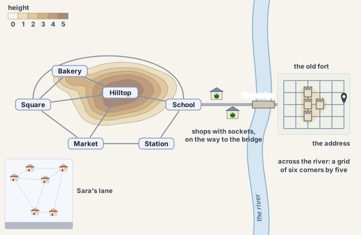
On Monday Sara has no bike, so she walks. Her phone finds the way to the Market before she has finished typing. Ines looks over her shoulder and laughs. “It knows the streets,” she says. “It doesn’t know this hill.” Sara wants to know what the phone actually worked out, and where it stops being right. The bus map from the Station is a good place to start. It shows the six places she has to know: the Bakery, the Square, the Market, the School, the Hilltop and the Station. It also shows the streets between them, but it says nothing about how long or how steep a street is. So the map answers the plainest question first. To reach the Market, how few streets can she get away with?
On Tuesday Ines lends her the old bike, and a street stops being just a street. The climb from the Bakery to the Hilltop takes seven minutes, but the ride back down takes three. Streets now take different times, so the way with the fewest streets and the quickest way are no longer the same.
The week after, the bakery’s e-cargo bike arrives. Its battery drains on the way up and fills again on the way down, so a ride downhill pays energy back. A street never takes negative time, but its cost in energy can be negative. The bike’s cargo box holds only so much, so on a busy morning Sara has to choose which orders go in. Each order brings a tip. Then comes an order from an address across the river. It is farther than the battery has ever gone, but the shops along the way have sockets.
And after the autumn there is a winter, with snow on every street of Sara’s own part of town and the neighbors deciding which ways through the gardens to dig first.
Little does Sara know that there is one underlying mathematical law that decides the best choice in all of her efforts.
Each of those days asks for the best choice, and each counts something else: streets, minutes, energy, the tips in a full box, the meters of snow to dig. The methods that answer them are close relatives, and the chapter takes the methods in that order. It ends on the question behind all of them. When can you choose the next step well without first working out the cost of everything after it?
6.2 The quickest way there
Breadth-first search and Dijkstra’s algorithm
On Monday the first order is for the Market. The bus map is in Sara’s hand, and the question is which way is quickest. On foot, with nothing but the bus map, every street counts the same. So the quickest way is the one with the fewest streets.
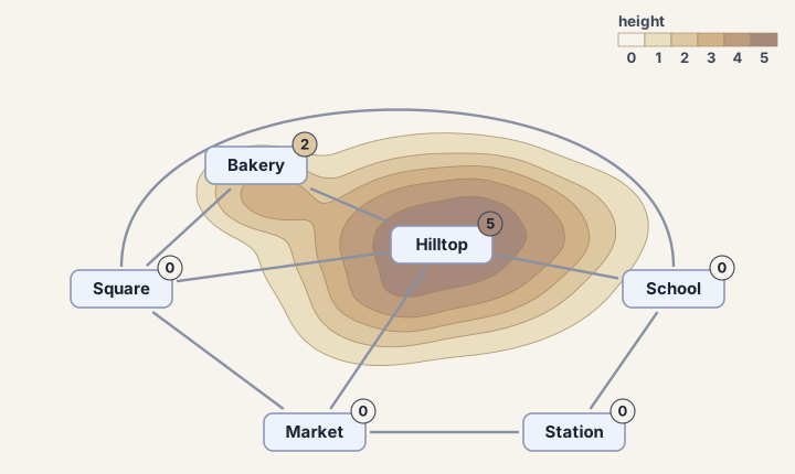
In the words of the graphs chapter, the places are the vertices of a graph, and the streets are its links. Each link joins two vertices both ways. A route is a path as the graphs chapter defines it. Such a path is a list of vertices with a link from each one to the next. A path may pass a vertex more than once. Here a path’s cost is the number of links on it.
6.2.1 Counting streets outwards
Breadth-first search
How can Sara find the fewest streets to every place at once? She works outwards from the Bakery. First she finds the places one street away: the Square and the Hilltop. Next she finds every place that lies one street beyond those and has not been found yet. Those are the Market and the School, both found from the Square. Last, she finds the Station from the Market. Each place is found once. When a place is found, Sara writes down the place just before it on the way.
In graph words, the vertex just before a found vertex is its previous vertex. Found vertices belong to the frontier until the search has looked along their links. They wait in a queue, the same kind of line that held the ready list in Kahn’s method in the graphs chapter. Whoever joined first is served first. The search takes the vertex at the front of the queue and looks along each of its links. Every vertex at the other end that has not been found yet joins the back of the queue. Each such vertex is one link farther from the start than the vertex that found it. On the map, the Square comes off the queue, and the Market and the School join the queue. Both are two streets from the Bakery. This is breadth-first search, BFS for short [1, Sec. 20.2].
| Taken from the front | Found now | Queue afterwards |
|---|---|---|
| Bakery (0) | Square (1), Hilltop (1) | Square, Hilltop |
| Square (1) | Market (2), School (2) | Hilltop, Market, School |
| Hilltop (1) | none | Market, School |
| Market (2) | Station (3) | School, Station |
| School (2) | none | Station |
| Station (3) | none | empty |
Call the number beside a place in Table 6.1 its count. Why is the first count for a place also its smallest? The answer lies in the order of the queue. In graph words, the queue hands out the vertices in order of their counts. Every vertex two links from the start comes off the queue before any vertex three links away, and the same holds for every count. A vertex is found from the first of its neighbors to come off the queue. Because of that order, this neighbor has the smallest count of all the vertex’s neighbors. So the first count for a vertex is its smallest. On the map, the Station is found from the Market, which is two streets from the Bakery. No neighbor of the Station is closer to the Bakery than the Market.
Looking along a link from vertex \(u\) to vertex \(w\) is one update of the count of \(w\), written \(c(w)\). The sign \(\leftarrow\) means that the right side replaces the left side. In the equation below, the first term inside the minimum keeps the count that \(w\) already has, and the second term offers a count through \(u\).
\[ c(w) \leftarrow \min\big( c(w),\ c(u) + 1 \big) \tag{6.1}\]
Every vertex begins at \(c = \infty\), except the start, which begins at 0. The code calls the count cost and writes None for \(\infty\). It needs no minimum, because a vertex’s first count is already its smallest.
Two facts hold the whole time. First, every vertex in the queue is at the count of the front vertex or one more. Second, the vertices at the smaller count stand in front. At first the queue holds only the start, so both facts hold. Taking the front vertex, at count \(k\), adds vertices at \(k + 1\) to the back. They stand behind every vertex at \(k\) and \(k + 1\) already there, so both facts still hold.
So vertices come off the queue in rings: every vertex at count \(k\) comes off before any at \(k + 1\). Write \(d\) for the fewest links on a path to a vertex \(v\), and take the vertex \(u\) just before \(v\) on such a path. For \(u\), the fewest links are \(d - 1\). Its count is \(d - 1\) too, by the same argument one ring earlier. When \(u\) comes off the queue, \(v\) is found if it has not been found already, so its count is at most \(d\). Can its count be less? No, because each count is the length of a real path, the one that the previous vertices trace back. So every count is the fewest links.
Following the previous vertices back gives the route itself. The Station was found from the Market, the Market from the Square and the Square from the Bakery. So the route is Bakery → Square → Market → Station, which is three streets long. Here it is in code. The whole module is bfs.py.
How much work does the search do? It takes each vertex off the queue once, and it looks along each of that vertex’s links once. So its work is \(\Theta(n + m)\) for \(n\) vertices and \(m\) links. Moore found the method for paths through mazes. Lee found the same method on his own and used it to route wires on circuit boards [1, p. 584], [2].
6.2.2 Minutes, not streets
Dijkstra’s algorithm
On Tuesday Sara rides. A street now takes minutes, and uphill takes longer than down. The street from the Bakery up to the Hilltop takes 7 minutes, and the way back down takes 3. In graph words, each street is now two arrows, one for each way, and each arrow has its own cost.
Key idea: costs and cheapest paths
In a weighted graph every arrow or link carries a number, its cost: minutes, meters, money, energy. The cost of a path is the sum of the costs of its arrows, and an arrow counts again each time the path uses it. A cheapest path from one vertex to another has the smallest cost of all the paths between them. There can be several, all with the same cost.
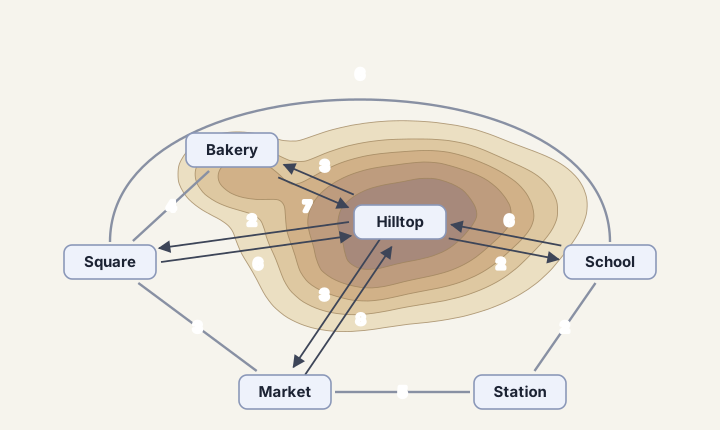
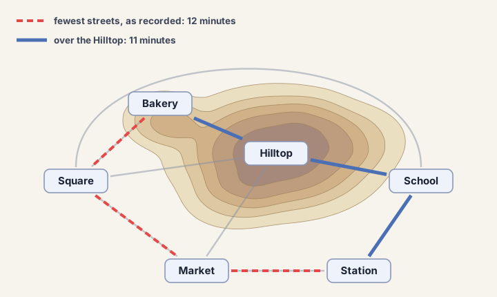
Counting streets is no longer enough. Breadth-first search found the Station by the route Bakery → Square → Market → Station, and that route takes \(4 + 3 + 5 = 12\) minutes. The route Bakery → Hilltop → School → Station has three streets too, and it takes \(7 + 2 + 2 = 11\) minutes (Figure 6.4). Both routes have three streets, so counting streets cannot tell them apart. The quicker one even climbs the hill, because the streets after the Hilltop take little time. On other maps, a route with more streets can be the quicker one.
Use the minutes in Figure 6.3, starting from the Bakery. Find the quickest time to every place. Then name the place, apart from the Bakery, whose quickest time is certain first, and say why.
Three minutes, on the map. You’re done when you have a time for every place, the place you were sure of first, and one sentence on why a route that you find later cannot beat it.
The same day, Sara switches the phone to the bike. It gives a time for any address the moment she types it, and Ines has to admit that the times are right. Counting streets cannot give those times, so the phone must work them out another way.
In graph words, every arrow now has a cost, and the search wants the cheapest path to every vertex. Breadth-first search found the vertices in rings, first those one link out and then those two links out. Now the rings have to grow by cost instead of by links. Call a vertex settled once the search has decided its cost and will never change it. The question is which vertex to settle next. At any moment the search knows a cost for some of the vertices, and each is the cost of a path it has actually found. Which of those costs is safe? A cost is safe when no other path to that vertex is cheaper.
Take the vertex with the smallest known cost among those not yet settled, and call it X. If several vertices tie, any of them will do, even one picked at random. Could some other path reach X more cheaply? No. The costs over the settled vertices are locked. Any other path leaves the settled vertices at some vertex Y that is not settled. Up to Y, that path costs at least Y’s known cost. Y’s known cost is at least X’s, because X was picked for the smallest known cost. A detour through any other vertex that is not settled cannot be cheaper, because no arrow costs less than 0.
Trying an arrow is the update of equation (6.1), with the arrow’s cost in place of the 1.
\[ c(w) \leftarrow \min\big( c(w),\ c(u) + \text{cost}(u \to w) \big) \tag{6.2}\]
As in breadth-first search, every vertex starts at \(c = \infty\), except the start, which begins at 0.
Always settling the vertex with the smallest known cost is the best-first search⬢ of the geometry chapter, run on a graph. The known costs wait in a priority queue, a structure that always hands out the smallest one first.
The promise rests on invariant 1. Invariant 2 is what makes it safe to settle the vertex with the smallest known cost next, and the priority queue hands that vertex out. The method keeps both invariants⬢ from start to end.
6.2.3 Settling one place at a time
The method in the box is Dijkstra’s algorithm [3]. What happens when a known cost drops? The search puts a new entry with the lower cost into the queue. The entry with the higher cost stays behind, and it is now an old entry. Because the new entry has the lower cost, it comes off first and settles the vertex. When the old entry comes off later, its vertex is already settled, so the search simply skips it. Keeping the old entries and skipping them is called lazy duplicates. Another kind of queue can find a vertex’s entry and lower its cost in place, so that queue never holds an old entry. Both kinds give the same costs [4, p. 399]. Neither kind is faster on every map. On roads and grids few arrows lower a known cost, so only a few old entries pile up there. Lowering an entry in place needs an index into the queue, and skipping the old entries costs less than keeping that index. This book’s code skips them, as NetworkX and petgraph do [5], [6]. Boost’s C++ Dijkstra lowers entries in place, with an index into its queue [7].
Here is the algorithm on Sara’s town, starting from the Bakery. The Market and the Hilltop tie at 7 minutes. The tie goes to the place named first in the bus map’s list, which is the Market.
| Step | Off the queue | Square | Market | School | Hilltop | Station | Queue afterwards |
|---|---|---|---|---|---|---|---|
| 1 | Bakery 0 | 4 | 7 | Square 4, Hilltop 7 | |||
| 2 | Square 4 | 4 | 7 | 10 | 7 | Market 7, Hilltop 7, School 10 | |
| 3 | Market 7 | 4 | 7 | 10 | 7 | 12 | Hilltop 7, School 10, Station 12 |
| 4 | Hilltop 7 | 4 | 7 | 9 | 7 | 12 | School 9, School 10, Station 12 |
| 5 | School 9 | 4 | 7 | 9 | 7 | 11 | School 10, Station 11, Station 12 |
| 6 | School 10, old | 4 | 7 | 9 | 7 | 11 | Station 11, Station 12 |
| 7 | Station 11 | 4 | 7 | 9 | 7 | 11 | Station 12 |
| 8 | Station 12, old | 4 | 7 | 9 | 7 | 11 | empty |
Watch step 4. The Hilltop is settled, and its arrow down to the School costs 2, so the School’s known time drops from 10 to 9. The School’s previous vertex changes from the Square to the Hilltop. At step 5 the Station’s previous vertex changes too, from the Market to the School. Following the previous vertices back from the Station gives the route Bakery → Hilltop → School → Station. That route goes over the Hilltop and takes 11 minutes.
Why is a cost final only once its vertex is settled? Breadth-first search never had to lower a count it had found, because its first count of a vertex was always the smallest. With costs, a vertex’s first cost can be beaten, as the School’s 10 was at step 4. So a cost becomes final only when its vertex is settled, as the bold entries in Table 6.2 show.
The queue in the code is Python’s binary heap. Its entries are pairs (cost, vertex), so a tie on cost goes to the smaller vertex number. The module is dijkstra.py.
The answer holds each vertex’s cost and its previous vertex. To read off the path to a vertex, step back through the previous vertices from that vertex to the start, then reverse the list of vertices you passed.
Here is why the method keeps the box’s two invariants.
At first only the start is known, at 0, and nothing is settled, so both invariants hold. The first vertex settled is the start, at 0. No path to it costs less than 0, since no arrow costs less than 0. Now suppose both invariants hold, and the method takes the unsettled vertex \(v\) with the smallest known cost \(d\). Take any path from the start to \(v\). It begins at the start, which is settled, so somewhere it must first reach a vertex \(x\) that is not settled. Every vertex before \(x\) on the path is settled. So by invariant 2 the part of the path up to \(x\) costs at least \(x\)’s known cost. The method picked \(v\) for the smallest known cost, so \(x\)’s known cost is \(\ge d\). The rest of the path costs \(\ge 0\), because the box’s Assumes says that no arrow costs less than 0. So the whole path costs at least \(d\). The path that the previous vertices give costs exactly \(d\). So settling \(v\) at \(d\) keeps invariant 1.
What about invariant 2? Settling \(v\) adds one vertex to the settled ones. A path whose earlier vertices are all settled can now end with an arrow out of \(v\). Trying every arrow out of \(v\), and keeping any lower cost, keeps invariant 2.
Breadth-first search is the same argument with every arrow costing one. Its queue then hands out the smallest count simply by keeping its order.
When every arrow counts as one, the simpler search is also the faster one. The New York road map of the DIMACS challenge has 264,346 vertices and 733,846 arrows, one for each direction in which a street can be driven. On it, breadth-first search took 0.29 of the time that Dijkstra’s algorithm took, for the same answer. On a random graph of a million vertices and four million arrows, and on a grid of a million vertices, it took 0.31 of Dijkstra’s time on each graph. Each time it gave the same answer. With the real lengths, though, most of its answers are wrong. On the New York map, 262,707 of the 264,346 vertices got a wrong route, and Dijkstra’s algorithm found a shorter route for each of them. For the median vertex the route was 16% longer, and for the worst vertex it was 82% longer. So the extra time buys Dijkstra’s algorithm the right answer.
Dijkstra’s algorithm also runs inside network routers. OSPF is one of the protocols that route traffic inside large networks. In OSPF, every router holds a map of the links and runs Dijkstra’s algorithm from itself to build its routing table [8, Sec. 16.1].
6.2.4 What it cannot do
The proof used one fact about the graph, written in the box as its Assumes: no arrow costs less than 0. On a graph with a negative arrow, Dijkstra’s algorithm can give a wrong cost. Why? The algorithm settles the vertex with the smallest known cost and never looks at that vertex again. A negative arrow tried later could still lower that cost, and by then it is too late. So settling a cost at once is what must go. The next method keeps trying every arrow until no arrow lowers a cost. Minutes are never negative, but next week Sara counts energy, and energy can be negative.
6.3 Downhill pays
The Bellman–Ford algorithm
The e-cargo bike arrives the next Monday. Ines shows Sara the battery gauge. Going uphill, the motor drains the battery. Going downhill, the motor works as a brake and charges the battery again. So on this bike Sara counts energy, because a flat battery halfway up the hill ends the trip. The phone knows how long the hill takes, but it has no idea what the hill does to the battery.
Here is how to price a ride in energy. Every place in town has a height. The energy of a ride along a street is its distance plus the height it climbs, and a drop counts as a negative climb. So a street between two places at the same height costs its distance both ways. The Bakery stands at height 2. The Hilltop stands at height 5, and the other four places stand at height 0. The ride from the Bakery up to the Hilltop covers a distance of 1 and climbs 3, so it costs \(1 + 3 = 4\). The ride from the Hilltop down to the Square covers a distance of 2 but drops 5, so it costs \(2 - 5 = -3\). A negative cost is no typo. Sara reaches the Square with more charge than she had on the Hilltop.
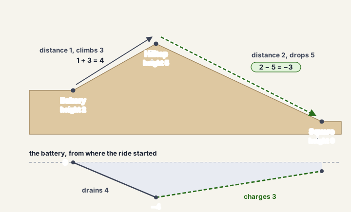
One warning before we go on. A total in energy says nothing about the battery’s size. A route with a small total can still run the battery flat on a long climb, before the drop that would have paid it back. This part ignores the battery’s size. Section Charge in the state comes back to it, by making the charge part of what the search remembers at each vertex.
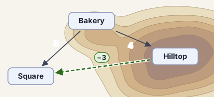
Here are three places of Sara’s town and three of its arrows, in energy (Figure 6.7): the Bakery to the Square costs 2, the Bakery to the Hilltop costs 4, and the Hilltop down to the Square costs \(-3\). Dijkstra’s algorithm from the last section settles the place with the smallest known cost first and never looks back. Run it from the Bakery. Say in one sentence whether you trust the cost it gives the Square.
Three minutes. You’re done when you have the cost it gives the Square and the sentence.
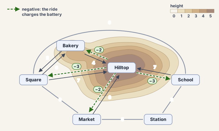
Figure 6.8 shows the whole town in energy. Sara starts at the Bakery, as before, and wants the cheapest way from there to every other place. Can we simply run Dijkstra’s algorithm on these costs?
In graph words, a negative cycle is a cycle whose arrows add up to less than 0. Many people believe that Dijkstra’s algorithm gives the right costs as long as the map has no negative cycle. Sara’s town has none. Every cycle comes back to the height at which it started, so its climbs and drops cancel, and only its distance is left, which is positive.
Yet Dijkstra’s algorithm fails here. From the Bakery it knows the Square at 2 and the Hilltop at 4. It settles the Square first, at 2, so that cost is final. Then it settles the Hilltop. The arrow down to the Square would give the Square \(4 - 3 = 1\), a better path. But the Square is already settled, so the algorithm skips that arrow, and the Square keeps 2. It is the only wrong cost in town, but the algorithm gives no sign of which cost is wrong, so the method cannot be trusted.
Which part broke? The proof in Settling one place at a time needed every arrow to cost \(\ge 0\), so that a path that leaves the settled vertices could only add cost. The arrow down from the Hilltop breaks that. Negative cycles had nothing to do with it.
So the smallest known cost is no longer safe to make final, since an arrow tried later might still lower it. The method of this section therefore settles nothing. It keeps trying every arrow, lowering costs whenever an arrow allows it, until no arrow lowers anything. Each try is the same update as in Dijkstra’s algorithm.
\[ c(w) \leftarrow \min\big( c(w),\ c(u) + \text{cost}(u \to w) \big) \tag{6.3}\]
Only the order and the number of the tries differ from those in Dijkstra’s algorithm. The question is whether the tries ever stop, and whether the costs are right when they stop. The tool for answering both is dynamic programming⬢.
Key idea: dynamic programming
Dynamic programming answers a large question from the answers to smaller questions of the same kind. Each smaller answer is worked out once and kept, so a question that many larger ones need is never solved twice. It needs an order in which every question comes after the smaller ones it uses.
You have already met it, in this chapter’s update equations. Breadth-first search (6.1), Dijkstra’s algorithm (6.2) and Bellman–Ford (6.3) each work out a vertex’s cost from the cost of the vertex just before it. The knapsack (6.5) will do the same.
Here a smaller question is the same question with fewer arrows allowed. For each vertex, ask for the cheapest cost of reaching it from the start with at most 1 arrow, then with at most 2, and so on. The design below runs these questions in rounds, where a round tries every arrow once. One more round at the end, the check round, tells whether the start reaches a negative cycle.
Why does the promise follow from the invariant? Pick any vertex \(v\), and assume the start reaches no negative cycle. Suppose a cheapest path from the start to \(v\) visits some vertex twice. The loop between the two visits is a cycle, so it costs \(\ge 0\), and cutting it out cannot make the path more expensive. Cut out every such loop and you get a cheapest path to \(v\) that visits no vertex twice. That path has fewer arrows than there are vertices. So after \(n - 1\) rounds, where \(n\) is the number of vertices, the invariant says that \(v\)’s cost is at most the cost of that path. The invariant also says that \(v\)’s cost belongs to a real path, and no real path to \(v\) is cheaper than the path without loops. The cost is therefore exactly the cheapest.
6.3.1 One more arrow at a time
To make the invariant precise, we count arrows. A path is a list of vertices with an arrow from each one to the next, and it may pass a vertex more than once. Write \(c_k(v)\) for the cheapest cost of a path from the start to \(v\) with at most \(k\) arrows. Think of \(c_k\) as row \(k\) of a table, with one column per vertex.
How do we get row \(k\) from row \(k - 1\)? Take a cheapest path to \(v\) with at most \(k\) arrows. If it has fewer than \(k\) arrows, it already counts in \(c_{k-1}(v)\). Otherwise its last arrow comes from some vertex \(u\). The part before that arrow is a cheapest path to \(u\) with at most \(k - 1\) arrows, because a cheaper one would make the whole path cheaper. So that part costs \(c_{k-1}(u)\). The cheaper of the two cases is \(c_k(v)\):
\[ c_k(v) = \min\Big( c_{k-1}(v),\ \min_{u \to v} \big( c_{k-1}(u) + \text{cost}(u \to v) \big) \Big) \tag{6.4}\]
The first term keeps every path with fewer than \(k\) arrows, as if the path waited at \(v\) for one step at no cost [9, Sec. 1.3.1], pp. 19–20.
Row 0 holds 0 for the start, which the path with no arrows reaches, and \(\infty\) for every other vertex. An offer from a vertex at \(\infty\) is \(\infty\) too, so it never wins the minimum. Filling each row from the one before is the dynamic programming of the key idea above. The code does not fill this table, but the table shows why the code’s tries of equation (6.3) work.
The Bellman–Ford algorithm [1, p. 644], [10], [11, Sec. 6.8] runs equation (6.4) with a single list instead of the whole table. The list holds one cost per vertex, the cheapest found so far. Each round goes through the vertices in a fixed order and tries every arrow out of each one. When an arrow \(u \to w\) offers \(w\) a lower cost, the list takes it at once, by equation (6.3), and records \(u\) as \(w\)’s previous vertex. When the rounds stop, following the previous vertices back from any vertex reads off a path with the cost that the list holds.
Because the list changes at once, a cost lowered early in a round is used later in the same round. So the list can run ahead of the table, but it never falls behind, as the box’s invariant says. Figure 6.9 shows the table and the list side by side.
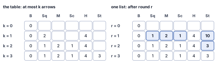
Watch round 1 on Sara’s town, where the order is Bakery, Square, Market, School, Hilltop, Station. The Bakery’s arrows go first, so the Square gets 2 and the Hilltop gets 4. The Square comes next and passes its 2 on, giving the Market 5 and the School 8. The Market then gives the Station 10, along Bakery → Square → Market → Station. The School’s arrow to the Station offers \(8 + 2 = 10\), which is no better. The round reaches the Hilltop only now. Its arrows down lower the Square to 1, the Market to 2 and the School to 1. Those are row 2’s costs, one round early, because the Hilltop’s 4 was already in the list when its turn came. The Station misses out in round 1, because the Market and the School passed their costs on before the Hilltop lowered them. Round 2 fixes that. The Market’s 2 lowers the Station to 7, and then the School’s 1 lowers it to 3. Round 3 lowers nothing.
Is running ahead safe? It is, and the reason is the box’s invariant, which holds in whatever order a round tries the arrows. The invariant has two halves. First, every cost in the list is the cost of a real path, since each write extends a real path by one real arrow. So no cost in the list can ever fall below the cost of a cheapest path. Second, after \(k\) rounds no vertex’s cost is above its \(c_k\). Take a vertex \(w\) and a cheapest path to \(w\) with at most \(k\) arrows. If that path has fewer than \(k\) arrows, then \(c_k(w) = c_{k-1}(w)\), and the earlier rounds already reached that cost. Otherwise call its last arrow \(u \to w\). Round \(k\) tries that arrow when \(u\) already holds at most \(c_{k-1}(u)\), because the earlier rounds saw to that. After the try, \(w\) holds at most \(c_{k-1}(u) + \text{cost}(u \to w)\), which is \(c_k(w)\). Running ahead only makes costs lower sooner, and that never breaks either half.
Now, when do we stop? The algorithm stops after a full round that changes nothing. The next round would try the same arrows from the same costs, so it would change nothing too, and the list can never change again. Such a list is a monotone fixed point⬢. Costs only ever go down, and when they stop going down, the list is the answer. In the graphs chapter, news passed around a group of people until it stopped spreading, and that end state was a monotone fixed point too.
But will the rounds stop? If the start reaches no negative cycle, yes. The argument after the box showed that \(n - 1\) rounds, for \(n\) vertices, already leave every cost at its cheapest. So the round after that changes nothing. If the start does reach a negative cycle, the costs around it can drop forever, and every round still lowers some cost. Why? Suppose a round lowered nothing. Then every vertex that the start reaches has a cost, because an arrow from a vertex with a cost to a vertex with none would give that vertex its first cost. Then every arrow \(u \to w\) of the negative cycle has \(c(w) \le c(u) + \text{cost}(u \to w)\). When you add up these inequalities around the cycle, the costs of the vertices cancel, and what is left says that the cycle’s total is \(\ge 0\). But a negative cycle has a total below 0. So one extra round tells the two cases apart. Without a negative cycle, that round changes nothing, and with a negative cycle it still lowers a cost. That extra round is the check round. If the check round still lowers a cost, the list cannot be the answer, and the algorithm reports a negative cycle instead. A negative cycle shows why that conclusion is right, and how to find the cycle from the previous vertices.
The work is easy to count. Every round tries every arrow once, so the work is the number of rounds times the number of arrows. Sara’s town has 18 arrows and needs 3 rounds, which makes 54 tries.
Here is one round in code. The module is bellman_ford.py. The round first copies the list it was given, so that each round returns a new state and leaves the old one intact. From then on it reads its own writes, so a cost lowered early in the round is used later in the same round.
The whole run repeats rounds until one lowers nothing. If the check round still lowers a cost, the run returns a negative cycle instead.
Here are the two halves in full.
First, every cost in the list is the cost of some path. Suppose this holds before a write, and the write goes along an arrow \(u \to w\). Then \(u\)’s cost is the cost of some path \(P\) to \(u\). The write gives \(w\) that cost plus the arrow, which is the cost of \(P\) followed by the arrow.
Second, after \(k\) rounds every vertex \(w\) holds at most \(c_k(w)\). We show it by induction on \(k\). After 0 rounds only the start has a cost, 0, which is \(c_0\). Now suppose the claim holds after \(k - 1\) rounds, and take a cheapest path to \(w\) with at most \(k\) arrows. Costs never rise, because a write only ever lowers one. If the path has fewer than \(k\) arrows, it counts in \(c_{k-1}(w)\), so \(w\) already holds at most that, and later writes can only lower it. Otherwise its last arrow is \(u \to w\). When round \(k\) tries that arrow, \(u\) holds at most \(c_{k-1}(u)\), so after the try \(w\) holds at most \(c_{k-1}(u) + \text{cost}(u \to w) = c_k(w)\). Nothing in this argument depends on the order of the arrows within the round [11, p. (6.26)].
6.3.2 A negative cycle
Sara’s town has no negative cycle, but other maps do. On the small map of Figure 6.11, the arrows from B to C, from C to D and from D back to B total \(1 - 4 + 2 = -1\). So each extra time around the cycle makes a path through it cheaper by 1.
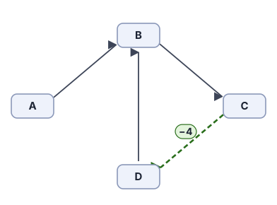
Start at A. Its one arrow goes to B and costs 2. Let each round go through the vertices in the order A, B, C, D. Run the rounds on this map and the costs never stop falling. After round 1, B, C and D cost 1, 3 and \(-1\). After round 2 they cost 0, 2 and \(-2\), and every round after that takes one more off each. Why does this show a negative cycle? Suppose there were cheapest paths. Then no loop on a path could have a negative total, because going round it once more would make the path cheaper still. So cutting a loop out of a path would never make it more expensive. Then some cheapest path to each vertex would pass no vertex twice. The map has four vertices, so such a path has at most three arrows. Three rounds would leave every cost at its cheapest, and the fourth round, the check round, would change nothing. But the check round still lowers a cost. So the start reaches a negative cycle. The answer is the cycle itself, read off the previous vertices as D → B → C → D, which is the same cycle as B → C → D → B.
The previous vertices form a picture with one pointer back from each vertex that has a cost. The pointer goes to the vertex whose arrow last lowered that cost. Take a vertex whose cost falls in the fourth round. The arrow from its previous vertex lowered it only because the previous vertex’s own cost had fallen since that arrow was last tried. So the previous vertex was lowered recently too. The same holds for its previous vertex, and so on back. Now follow the previous vertices back from the last vertex that the fourth round lowered, for as many steps as there are vertices. You land on a cycle of previous vertices [12], and every cycle that the previous vertices close has a negative total [1], Lemma 22.16 and its proof, pp. 635–637. Then keep stepping back from the vertex where you landed until you reach it again. The vertices you pass, in reverse order, are the cycle.
Routers that know only their neighbors use Bellman–Ford’s tries, again and again. In RIP, each router tells its neighbors the costs it knows. A router takes the cost that a neighbor has for a destination and adds the cost of the link to that neighbor. When this sum is lower than the router’s own cost for that destination, the router takes the sum as its new cost. These are Bellman–Ford’s tries, but the routers share no rounds. Each router sends on its own clock, about every 30 seconds, and the protocol keeps the clocks from falling into step [13, Sec. 3.8]. Babel is a newer protocol of the same kind. It adds a condition on which routes a router may accept, so that its routes never form a routing loop [14, Sec. 2.4].
On the New York road map of the DIMACS challenge, where no street costs less than 0, Bellman–Ford needed 614 rounds and 450 million tries of an arrow, for an answer that Dijkstra’s algorithm got by trying each arrow once. Bellman–Ford took about 65 times as long. The number of rounds decides the gap. On a random graph of 100,000 vertices and 400,000 arrows, Bellman–Ford stopped after 15 rounds and took 1.25 times Dijkstra’s time. On a grid of 90,000 vertices, it needed 62 rounds and took 5.3 times as long. With some negative arrows, Dijkstra’s algorithm stays about as fast, but its answer becomes wrong. On the New York map, a height per vertex made 318,533 arrows negative. Dijkstra’s algorithm then gave 262,874 vertices a cost that was too high.
6.3.3 What it cannot do
A negative cycle leaves no cheapest path to the vertices on it, so all the algorithm can do is report the cycle. The rounds are also slow. On a graph of \(n\) vertices and \(m\) arrows they cost \(O(nm)\), while Dijkstra’s algorithm costs \(O(m \log m)\). The logarithm comes from its priority queue, where each push or pop takes \(O(\log m)\) steps (appendix).
When a map has negative arrows but no negative cycle, there is a way to make Dijkstra’s algorithm run on it after all, by giving every vertex a height that changes the costs so that none is negative (appendix).
Some maps do not need the rounds at all. When a map has no cycle, one pass in topological order gives the same costs as all the rounds. That is how the news reached Omar in the graphs chapter. The next problem becomes a graph with no cycle.
6.4 What fits in the box?
Knapsack as a longest path
The e-cargo bike has a box that holds 10 kilograms. On Thursday three orders wait at the counter. A birthday cake weighs 5 kilograms and brings a tip of 10. Bread for the school kitchen weighs 4 kilograms and brings a tip of 7. Pastries for a café weigh 6 kilograms and bring a tip of 11. There is time for only one trip before the orders are due. Whatever does not fit waits for Ines’s van in the afternoon, and the tips go with whoever delivers.
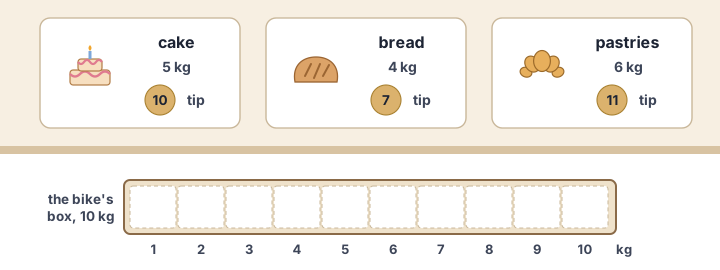
Pick the orders that fit in the 10 kilograms for the most tips.
Two minutes. You’re done when you can say your pick, its tips, and why no other pick beats it.
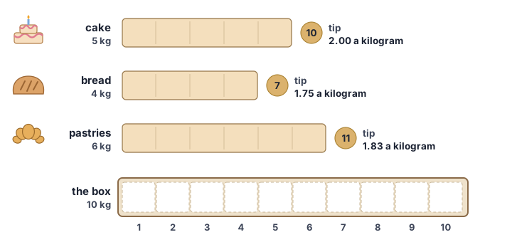
Ines has done this every morning for eleven years. As Sara loads the bike, Ines offers her rule of thumb. The orders whose tips pay best for their weight go in first.
Many people use this rule. The cake brings 2 in tips for each kilogram. The pastries bring about 1.83 in tips for each kilogram, and the bread brings 1.75. So the cake goes in first. The pastries no longer fit, but the bread does, for 9 kilograms and 17 in tips. Yet the bread and the pastries weigh exactly 10 kilograms and give 18. The rule left a kilogram of the box empty.
Each order is either in the box or not, so three orders give \(2 \times 2 \times 2 = 8\) picks, and Sara could try all eight. Thirty orders give \(2^{30}\) picks, more than a billion. So what does she need to know after each order, to decide the rest well? She needs to know only how much of the box the orders have used so far. Two picks that weigh the same leave the same room, so the one with more tips so far is the better start.
Sara’s problem is the knapsack problem, named after a hiker’s bag. In general it has \(n\) items, each with a weight and a value, and one capacity. It asks for the items whose total weight fits the capacity and whose total value is the largest. Here the orders are the items, and their tips are the values. Their kilograms are the weights, and the box’s room is the capacity.
The state after each decision is then a pair: how many items are decided, and how much weight is used. From each state with an item still to decide, one arrow skips that item and gains nothing. A second arrow takes the item and gains its value. That arrow exists only if the item fits in the capacity left. The start is the state with nothing decided and nothing used. Every path from the start to a state with every item decided is one pick that fits, and the values that the path gains add up to its length. On Sara’s Thursday the states and the arrows form a graph, and the graph holds every way that the morning could go. Following one path simulates one of those mornings, and order by order you watch the tips pile up and the kilograms fill the box.
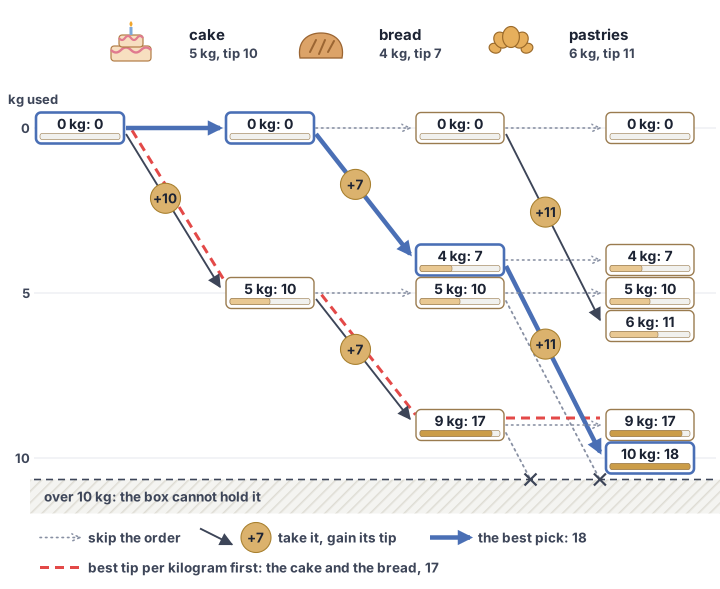
Take the state “4 kg: 7” in the third column of Figure 6.14. Two orders are already decided here. The cake is skipped, and only the bread is in the box, so 4 kilograms are used and the tips are 7. Only the pastries are left to decide. From that state, one arrow skips them and keeps 4 kilograms. The other takes them and leads to 10 kilograms and 18 in tips.
The best pick is the longest path in this graph, the one whose arrows gain the most. Turning the items into this graph is a reduction⬢, as 2-SAT was in the graphs chapter. A question about items and a capacity becomes a question about paths. Count every value as a negative cost, and the longest path becomes the cheapest path, which Bellman–Ford already finds.
The graph has no cycle, because every arrow decides one more item. That makes the longest path easy to find. Group the states by how many items are decided, and call each group a layer. Every arrow into a state of layer \(i\) comes from layer \(i - 1\). So you can fill the layers one at a time. Each state takes the best of the one or two arrows into it, and one pass gives every state its longest path.
Trying an arrow into a state is the update of equation (6.2), with a maximum in place of the minimum, because values are gained.
\[ t(w) \leftarrow \max\big( t(w),\ t(u) + \text{value}(u \to w) \big) \tag{6.5}\]
Here \(t(w)\) is the largest value found so far at the state \(w\). Every state except the empty start begins at \(-\infty\), which the code writes as None. The empty start begins at 0. This is dynamic programming again. The knapsack’s answers fill a dynamic-programming table, a DP table for short. It has a column for each layer, as in the graph, and a row for each weight from 0 to the capacity. Figure 6.15 shows this DP table.
In the DP table a state \(w\) is a cell \((i, k)\): the layer \(i\) and the weight used, \(k\). Write \(\text{weight}_i\) and \(\text{value}_i\) for the weight and the value of item \(i\). Two arrows lead into \((i, k)\). The arrow for skipping item \(i\) comes from the cell to its left, \((i - 1, k)\). The arrow for taking item \(i\) comes from the cell \((i - 1, k - \text{weight}_i)\) and adds \(\text{value}_i\). So equation (6.5) for one cell reads
\[ t(i, k) = \max\big( t(i - 1, k),\ t(i - 1, k - \text{weight}_i) + \text{value}_i \big) \tag{6.6}\]
where the second term counts only when the item fits, \(k \ge \text{weight}_i\).
In the code each layer is a list with one entry per unit of weight, and an entry is None at a weight that no pick reaches. The code calls the weight used w, where the DP table says \(k\). This w is a weight, not the state \(w\) of equation (6.5). The code also calls a state’s largest value so far its gain. It tries each state’s two arrows, and the state at the end of an arrow keeps whichever is larger, its own gain or the gain that the arrow brings. The module is knapsack.py.
The pick itself comes from stepping back from the best state, one layer at a time. At each layer, ask whether taking the item could have given this state’s gain. If it could, the item is in the pick. When taking and skipping give the same gain, the item goes in the pick too.
Every arrow decides one item, so a path from the start to layer \(n\) decides each of the \(n\) items once. The path can take an item only if the item fits, so the pick that it makes fits the capacity. The path’s length is the sum of the values of the items it takes. Now start with a pick. A pick that fits gives one path: skip or take each item in turn, and the weight used never passes the capacity. So paths and picks match one to one, and the longest path is the best pick. No arrow goes back a layer, so the graph has no cycle, and its longest path is well defined.
The same move works on words. Turning one word into another by inserting, deleting and changing letters is a path through a grid, and the fewest such edits make a cheapest path. Exact DNA aligners search that grid for the fewest edits between two sequences [15]. By default, git diff searches it with inserts and deletes only [16], [17]. The studio chapter builds that grid.
6.4.1 The capacity DP table
This chapter’s DP table has a value in a cell only when some pick weighs exactly that cell’s weight. Call it the exact-weight DP table. Most textbooks fill another one. Its cell at weight \(k\) holds the largest value of a pick that weighs \(k\) or less, so it answers the knapsack for a box of capacity \(k\). Call it the capacity DP table. One line fills both tables, equation (6.6). Only the first column differs. Put 0 only at weight 0, and the line fills the exact-weight DP table. Put 0 in every cell of the first column, and it fills the capacity DP table (Figure 6.16).
In the capacity DP table a cell often gets a value from both of its arrows. At 10 kilograms in the last layer, skipping the pastries brings 17 in tips. Taking them adds their 11 to the 7 that the bread alone brings at 4 kilograms, for \(7 + 11 = 18\) in tips. The maximum keeps the larger, so the cell holds 18. In the exact-weight DP table, with these three orders, a cell gets a value from one arrow at most, because no two picks weigh the same.
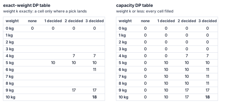
The capacity DP table also follows from the exact-weight one, column by column. Go down a column and keep the largest value so far. In the last layer at 7 kilograms, the exact-weight DP table offers 0, 7, 10 and 11 up to that row, so the capacity DP table holds 11.
The capacity DP table is the easier one to code. No cell in it is ever empty, and its last column answers every smaller capacity with one cell for each. The exact-weight DP table knows more, because it shows which weights some pick can reach, and the capacity DP table follows from it in one pass. And when few weights are reached, the exact-weight DP table can keep only those.
6.4.2 What it cannot do
Each layer of the graph can have one state for every weight up to the capacity. So the graph grows with the capacity, not only with the number of items. A box of 10 kilograms is easy. A cargo hold measured in grams, with weights up to a billion grams, is not easy. When the weights are large numbers, the approximation chapter gives up a little of the best value to keep the graph small.
Life can only be understood backwards; but it must be lived forwards.
after Søren Kierkegaard, journal (1843)
6.5 What is this all about?
Bellman’s equation
Four problems so far use the same update, in equations (6.1), (6.2), (6.3) and (6.5). Each update looks one arrow further, so you can count the steps, as in equation (6.4). A step is one arrow on a path, and in the knapsack a step decides one item. Write \(c_k(v)\) for the cheapest cost of reaching \(v\) in at most \(k\) steps. In the DP table’s view, \(k\) counts the items decided, and \(v\) is the weight used.
\[ \begin{aligned} &c_0(\text{start}) = 0, \qquad c_0(v) = \infty \text{ for every other } v,\\ &c_k(v) = \min\Big( c_{k-1}(v),\ \min_{u \to v} \big( c_{k-1}(u) + \text{cost}(u \to v) \big) \Big) \end{aligned} \tag{6.7}\]
This is Bellman’s equation [10], [18], in the form for this chapter’s problems. Its first term is there because in path problems a path can wait at a vertex for a step at no cost, and in the knapsack an item can be skipped. Without such a move, the equation would have only the second term. Look at the two sides. On the left is the question for \(v\) in at most \(k\) steps. On the right are the same questions with one step fewer, for \(v\) itself and for the vertices just before \(v\). So the equation answers a question from the answers to smaller questions of the same kind, and that is dynamic programming. Bellman–Ford and the knapsack fill in these answers one round or one layer at a time. The other methods reach the final answers in another order, and that order decides which costs each method can trust.
No cheapest path needs more steps than there are vertices, unless a negative cycle is reachable. After that many steps, one more step changes nothing, so you can drop the index \(k\). Every cheapest path to a vertex other than the start ends with an arrow, so the first term can go.
\[ c(\text{start}) = 0, \qquad c(v) = \min_{u \to v} \big( c(u) + \text{cost}(u \to v) \big) \text{ for every other } v \tag{6.8}\]
This form without steps is Bellman’s equation too, the one in his routing paper [10].
Dijkstra’s algorithm solves equation (6.8) directly, in order of cost, because no arrow is negative.
Equation (6.8) also says that every piece of a cheapest path is itself a cheapest path. Notice which way the equation reads. It looks backwards, from the end of a path to its start. Every method so far solves it forwards, from the start outwards.
Now read the same equation from the goal instead. It then gives \(r(u)\), the cost still to go from a vertex \(u\) to the goal.
\[ \begin{aligned} &r(\text{goal}) = 0,\\ &r(u) = \min_{u \to v} \big( \text{cost}(u \to v) + r(v) \big) \text{ for every other } u \end{aligned} \tag{6.9}\]
In the sum, \(\text{cost}(u \to v)\) is the next step. \(r(v)\) is the rest of the way, the cost of everything after that step. So when can a method choose the next step without knowing the rest of the way? That depends on how much the method knows about \(r(v)\). What these are actually made of answers this for each method (Table 6.6).
What tells the methods apart? It is the order in which they solve Bellman’s equation (Table 6.3).
| Method | Order of solving |
|---|---|
| breadth-first search | one arrow further at a time and each vertex once, which is Dijkstra’s order when every arrow costs 1 |
| Dijkstra’s algorithm | the smallest known cost first, each vertex once |
| Bellman–Ford | every arrow, in rounds, until a round changes nothing |
| in topological order | each vertex after every vertex with an arrow into it |
A graph with no cycle can be put in a topological order⬢, so that every arrow points forward. The graphs chapter built such an order with Kahn’s method. Take the vertices in that order. Then every arrow into a vertex has been tried before the vertex is taken, so one pass gives every cost. The knapsack’s layers already come in topological order, so one pass is enough there too. That order is the last row of Table 6.3.
The library’s method takes Kahn’s order and tries each vertex’s arrows once. It skips a vertex that no arrow has reached. Arrows may be negative here, because every arrow into a vertex is tried before the vertex is taken [1, Sec. 22.2]. A graph with a cycle has no such order. There the method returns the vertices that Kahn’s method could not put in order. The module is dag.py.
Here are the methods so far, side by side. Each one promises something different, at a different cost (Table 6.4).
| Method | Promise | Cost | Assumes |
|---|---|---|---|
| breadth-first search | the fewest arrows to every vertex | \(\Theta(n + m)\) | every arrow counts one |
| Dijkstra’s algorithm | the cheapest path to every vertex | \(O(m \log m)\) | no negative arrow |
| Bellman–Ford | the cheapest paths, or a negative cycle | \(O(nm)\) | none |
| the knapsack as a longest path | the best pick that fits | \(\Theta(nC)\) | integer weights \(\ge 0\) |
The next order is a single address on the far side of the river. On that side the streets form a grid, and every block takes at least 2 minutes. Dijkstra’s algorithm settles the places in order of time, so it would first settle every place that is nearer in time than the address. Without riding there, what could you say for sure about the time still to go from any corner? And where in Dijkstra’s algorithm would you use that number?
Five minutes. You’re done when you can name one such number, say why it is never too large, and say how Dijkstra’s algorithm would use it to pick the next corner.
6.6 Heading for the address
A* search
On Saturday the order is for an address across the river. On that side the streets run in a grid of six corners by five. A corner here is any place where two streets of the grid cross, not only one of the grid’s four outer corners. Each block takes 2 minutes, with one exception. The old fort has four towers, each on a corner of the grid, and Figure 6.17 marks where they stand. A block that climbs to a tower takes 5 minutes, even from another tower. A block that leads down from a tower to a corner with no tower takes the usual 2 minutes. Sara starts where the bridge comes in, at the middle of the grid’s west side. The address is in the middle of its east side.
What does Dijkstra’s algorithm do here? When it runs from the bridge, it settles the corners in order of time, and time grows the same way in every direction. So it settles the corners beside Sara just as early as the ones ahead. On this grid it settles all 30 corners, and the address is the last.
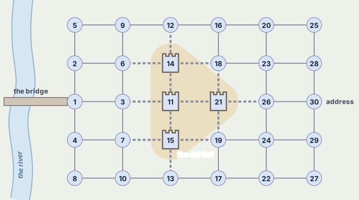
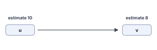
But Sara knows something that Dijkstra’s algorithm does not use. From any corner, the address is a certain number of blocks away, and every block takes at least 2 minutes. So 2 minutes for each block still to go is a time she cannot beat from that corner. It is a lower bound on the rest of the way⬢. Like a region’s bound in the geometry chapter’s best-first search, it never claims too much. In graph words, such a lower bound on the cost still to go from a vertex \(v\) is its estimate, written \(h(v)\). Each vertex has one estimate, and the estimate never changes during the search.
You choose the estimate \(h\), in any problem. A good one is
- safe: it never claims too much, and along any arrow it drops by no more than the arrow costs, as the box below asks;
- close: the nearer it comes to the real cost still to go, the fewer vertices A* settles;
- quick: A* works it out at every vertex that it reaches [19, Sec. 3.6].
To find one, drop a rule of the problem and take the cheapest cost still to go in the easier problem. Such a cost never claims too much, and it keeps the invariant [19, Sec. 3.6.2]. Sara’s estimate drops the fort’s slow blocks.
The invariant is what lets Dijkstra’s box apply, as the next section shows.
6.6.1 The same search, on changed costs
Here is the trick. Give every arrow a changed cost, \(\widehat{\text{cost}}(u \to w) = \text{cost}(u \to w) + h(w) - h(u)\). The invariant says that the estimate drops by no more than the arrow costs, so no changed cost is negative. Add up the changed costs along a path from the start to the goal. The estimates cancel at every vertex in between:
\[ \begin{aligned} \text{changed cost of the path} &= \text{cost of the path} + h(\text{goal}) - h(\text{start})\\ &= \text{cost of the path} - h(\text{start}) \end{aligned} \tag{6.10}\]
where \(h(\text{goal}) = 0\). So every path to the goal changes by the same amount, and the cheapest one stays the cheapest. That makes Dijkstra’s algorithm on the changed costs correct, as the design 6.1 promises. Dijkstra’s algorithm on these costs is called A* search [20]. Write \(\hat c(w) = c(w) + h(w)\) for a vertex’s known cost plus its estimate. With the changed costs, Dijkstra’s update, equation (6.2), becomes
\[ \hat c(w) \leftarrow \min\big( \hat c(w),\ \hat c(u) + \widehat{\text{cost}}(u \to w) \big) \tag{6.11}\]
Take \(h(w)\) away on both sides, and this is equation (6.2) again. So every vertex that A* settles gets Dijkstra’s cost. Only the order of the queue changes, because the queue takes the smallest \(\hat c\) first.
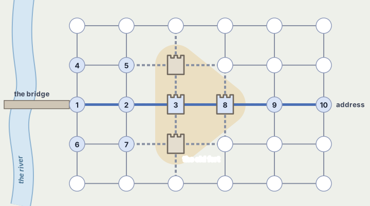
How much does the estimate save? With the estimate at 2 minutes for each block to go, A* settles 10 corners on the grid instead of 30. It reaches the address in the same 16 minutes that Dijkstra’s algorithm finds, by the route straight over the fort: \(2 + 5 + 5 + 2 + 2 = 16\). Why does it settle any corner off that route? The estimate cannot see the fort’s slow blocks. So A* also settles a few corners beside the straight route, where a way around the fort might begin. A* finds that the climb is still the quicker way only after it settles them. Past the fort the estimate falls exactly as fast as the time, so A* goes straight to the address.
A queue entry’s priority is the number by which the queue orders its entries. In A* it is \(\hat c\), and the code calls it key. The code is Dijkstra’s algorithm with each entry’s priority raised by the estimate. It stops as soon as the goal is settled. So only the costs of the goal and of the vertices settled before it are final. The other vertices keep whatever cost the search knew when it stopped. The module is a_star.py.
No. Take an estimate that never claims too much. Along some arrow it can still drop by more than that arrow costs. Then some changed cost is negative, and Dijkstra’s box no longer applies. A vertex can be settled too early, just as the Square was in Figure 6.7.
A* never settles more vertices than Dijkstra’s algorithm, when the estimate keeps the box’s invariant and ties go by the vertex’s number [21], Thm 4.1. How many fewer vertices it settles depends on how much the estimate knows. An estimate of zero everywhere keeps the invariant too, and with it A* is Dijkstra’s algorithm. If every arrow also costs 1, it finds the fewest arrows to the goal, as breadth-first search does.
The New York road map gives measured numbers for 100 trips between random vertices. In this test both searches stopped as soon as they settled the goal. A* with a straight-line estimate settled 44% of the vertices that Dijkstra’s algorithm settled. A* took 55% of the time that Dijkstra’s algorithm took, 4.1 ms a trip against 7.4 ms.
The estimate was the straight-line distance to the goal, times the smallest cost per unit of straight line among the map’s arrows. So it keeps the box’s invariant, and no street of the map breaks it. Dijkstra’s algorithm stopped as soon as the goal was settled, as A* does. On a grid of a million vertices where every arrow costs one, A* settled 22% of the vertices that Dijkstra’s algorithm settled and took 17% of its time. Where does it lose? Take the same grid with arrow costs from 1 to 1000. The estimate counts every arrow at the cheapest arrow’s cost, which says almost nothing about the real cost. So A* settled nearly as many vertices as Dijkstra’s algorithm, and it took 5% longer than Dijkstra’s algorithm because of its extra work per step.
6.6.2 Charge in the state
The battery has a limit, and the trip across the river is longer than one charge. The shops along the way have sockets, and Ines lets Sara stop at any of them. Now the best route depends on more than where she is. Picture two visits to the same corner, one with a full battery and one with an empty one. They lead to different futures.
So the state remembers the charge⬢, just as the knapsack’s state remembered the weight used. A state of the new graph is a pair, a vertex and a charge level. An arrow from one vertex to the next leads from the pair (vertex, charge) to (next vertex, charge minus the energy that the arrow uses). The arrow is there only when the new charge is at least zero. When an arrow downhill would raise the charge past full, the charge stops at full, because a full battery takes no more. At a vertex where charging is possible, one more arrow leads from (vertex, charge) to (vertex, charge plus one level). It costs the time that the charging takes. The cheapest path in this graph is the quickest trip that never runs the battery flat. Dijkstra’s algorithm and A* run on this graph unchanged.
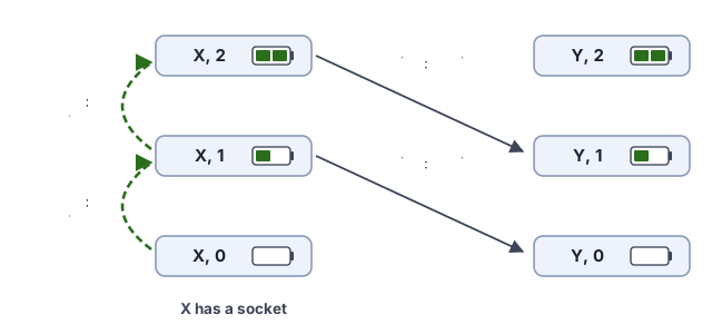
Electric-car routing does the same. One published method keeps a copy of each charging station for each battery level at which a car may arrive. It then runs Dijkstra’s algorithm or A* on the larger graph [22]. Parking robots and self-driving cars plan with hybrid A*, whose states are positions together with the direction that the car faces [23]. The open-source planners Nav2, Apollo and Autoware ship it [24], [25], [26].
6.6.3 What it cannot do
What can go wrong? An estimate that claims too much, or that drops by more than an arrow costs, can make A* return a path that is not the cheapest. A real library, petgraph, shipped that fault [27]. A check among the hands-on projects asks you to find it. A second limit is that A* needs one goal. When the search must reach every vertex, no estimate helps, and Dijkstra’s algorithm is the method.
A street can close while Sara is on her way. Then the answer that she had is about a map that no longer exists. The fix is to ask again from where she is, on the map as it is now. That costs a whole new search for every change. D* Lite asks again without starting over. It works from the goal and recomputes only the costs still to go that changed and that matter for the way ahead [28, pp. 2, 4].
The winter’s question changes what a step costs. When the aim is to join everyone, a step costs the link alone, not the cost so far plus the link.
6.7 After the big snow
Spanning trees: Kruskal’s and Prim’s algorithms
In January the snow comes all at once, and by morning Sara’s own street is buried. The plow clears the main road. It leaves a wall of snow along the road, broken only at Hana’s drive. Six households live along the lane behind the road. Grandma lives at the end, and the others are Sara’s family, Yusuf, Elena, Tomás and Hana. At eight they call to each other over the garden fences, spades ready, and agree on one thing. Every household must be able to reach every other household, because Grandma needs visits and Hana’s car is the only one that starts. And nobody wants to dig a meter more than that.
They know the gardens. Between some pairs of houses the way through is short, and between others it is long. Some pairs have no gate at all. Sara writes down the meters.
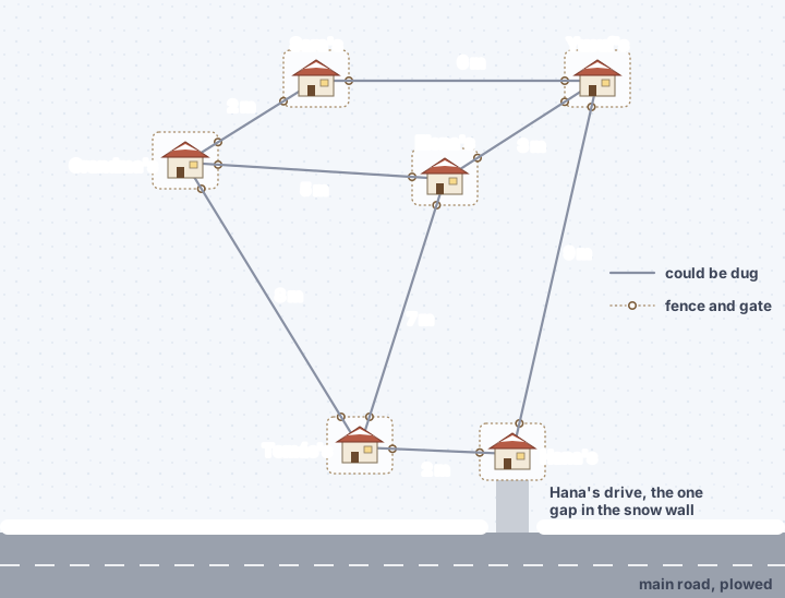
Which trenches would you dig, so that every household can reach every other household?
Three minutes. You’re done when you can say your trenches, their total, and why no plan digs less.
The first plan in the lane is that everyone digs to their nearest neighbor. Grandma and Sara’s family are 2 meters apart, Yusuf and Elena are 3 meters apart, and Tomás and Hana are 2 meters apart. Each pair digs its trench. The result is three islands. Nobody can get from one island to another, because no dug trench leaves an island.
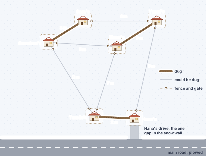
In graph words, the households are vertices, and each trench is a link whose cost is its meters. The lane asks for the cheapest set of links that joins every vertex.
Key idea: spanning trees
A spanning tree of a connected graph is a set of its links that joins every vertex and closes no cycle. With \(n\) vertices it has \(n - 1\) links. A minimum spanning tree is one with the least total cost. When links tie, there can be several, all with the same total. A graph in several pieces has one tree per piece, and together they form a spanning forest.
Is this the summer’s problem again? It can be written the same way. Suppose some vertices are already joined. Each link out of the joined group gives a sum of two costs. The first is the link’s own cost. The second is the cost of joining the remaining vertices, once the group also holds the link’s other end. The cost to join every vertex is the smallest of these sums. That is Bellman’s equation again, with the joined group as the state. There are too many groups to try them all. But here the second cost can be skipped. One link out of the group is always safe, whatever the rest costs.
Which link out of a joined group is always safe to keep?
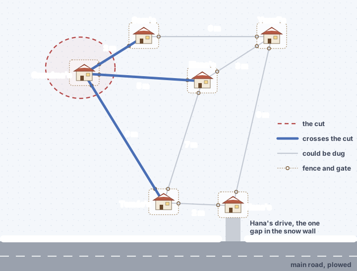
Split the vertices into two sides, any way you like. Call such a split a cut. Every spanning tree has at least one link across the cut, or the two sides could never reach each other. Now take a minimum spanning tree that does not use the cheapest link across the cut. Add that link too, and the tree now has a cycle. The cycle crosses the cut at least twice, because whatever crosses to one side has to come back. One crossing is the cheapest link, \(e\). Some other link of the cycle also crosses the cut, and that link costs at least as much as \(e\). Remove that other link. Every vertex is still joined, because the cycle still goes around the other way. And the total does not go up. This swap of one link for another is an exchange. So the cheapest link across any cut is in some minimum spanning tree. This is the cut property. The joined group and the rest are one such cut, so the cheapest link out of the group is always safe.
The promise rests on invariant 1. Invariant 2 lets the algorithm test whether a link closes a cycle, and each test takes nearly constant time.
6.7.1 The cheapest first, unless it closes a cycle
Kruskal’s algorithm
Kruskal’s algorithm [29] takes the links cheapest first. If a link’s two ends are not yet joined, it keeps the link. If they are joined already, it skips the link, because that link would close a cycle. So the algorithm keeps asking whether a link’s two ends are already joined. Union-find, the structure of the graphs chapter, answers that question, so each test takes nearly constant time. In the lane, equal lengths go in the order in which Sara wrote them down.
| Link | Meters | Kept? | Groups afterwards |
|---|---|---|---|
| Grandma–Sara | 2 | yes | {Grandma, Sara}, Yusuf, Elena, Tomás, Hana |
| Tomás–Hana | 2 | yes | {Grandma, Sara}, Yusuf, Elena, {Tomás, Hana} |
| Yusuf–Elena | 3 | yes | {Grandma, Sara}, {Yusuf, Elena}, {Tomás, Hana} |
| Grandma–Elena | 5 | yes | {Grandma, Sara, Yusuf, Elena}, {Tomás, Hana} |
| Sara–Yusuf | 6 | no, both ends joined already | unchanged |
| Elena–Tomás | 7 | yes | everyone |
Why is every kept link safe? When Kruskal’s algorithm keeps a link, look at the group on one of its ends, and cut that group off from every other vertex. Every cheaper link came earlier. Once its turn had passed, its two ends were in one group, and groups only merge. So no cheaper link crosses this cut. The kept link is therefore a cheapest link across the cut, and by the cut property it is safe. That is the exchange argument⬢ at work. Any minimum spanning tree can be turned into the tree that Kruskal’s algorithm builds. Each step swaps one link, and no swap raises the total.
Now go back to the first plan in the lane, where everyone dug to the nearest neighbor. A household’s nearest link is the cheapest link across the cut between that household and everyone else. So by the cut property each of the plan’s three links was safe, and Kruskal’s algorithm kept all three (Table 6.5). The plan was not wrong. It just stopped at three islands, and Kruskal’s algorithm goes on to join them.
Here it is in code. The module is kruskal.py.
Take a minimum spanning tree \(T\) and a cut, and let \(e\) be the cheapest link across the cut. If several links tie for cheapest, \(e\) is any one of them. If \(T\) holds \(e\), there is nothing to show. Otherwise adding \(e\) to \(T\) closes exactly one cycle. That cycle crosses the cut an even number of times, because every crossing over has to be matched by a crossing back. So some other link \(f\) of the cycle crosses the cut too. Since \(e\) is the cheapest link across the cut, \(f\) costs at least as much as \(e\). Remove \(f\). The result still joins everything, because the cycle still connects \(f\)’s two ends. The result has one link fewer than there are vertices, so it is a spanning tree. And its total is at most \(T\)’s total. So some minimum spanning tree holds \(e\) [1], Thm 21.1, p. 587.
For Kruskal’s algorithm, invariant 1 follows. When it keeps a link, let the cut separate the group on one end from everything else. No earlier kept link crosses that cut. The reason is invariant 2. Two vertices are in one group exactly when the earlier kept links join them, so every earlier kept link has both ends in one group. Every cheaper link was already looked at. A kept one does not cross the cut. A skipped one had both ends joined already, so it does not cross either. So the link being kept is the cheapest link across that cut. By invariant 1 some minimum spanning tree \(T\) holds the earlier kept links. Run the exchange above on that \(T\). It removes a link \(f\) that crosses the cut, so \(f\) is never an earlier kept link. The kept links and the new one together stay part of some minimum spanning tree.
6.7.2 From Grandma’s door
Prim’s algorithm
Grandma, at the end of the lane, has her own plan. She starts digging at her door. Then, again and again, she digs the shortest trench from the households already joined to a household not yet joined. Sara’s family comes first, because they are only 2 meters away. Then come Elena from Grandma at 5 meters, Yusuf from Elena at 3 meters, Tomás from Elena at 7 meters and Hana from Tomás at 2 meters. Her plan has the same five links as Kruskal’s algorithm and the same 19 meters, but she digs the links in another order. This is Prim’s algorithm [30]. In graph words, it grows one tree from a start vertex and always adds the cheapest link from the tree to a vertex outside it. Why is it safe? Every link that it adds is the cheapest across the cut between the tree’s vertices and the rest. So the cut property makes it safe too.
The code looks like Dijkstra’s algorithm, and it is Dijkstra’s algorithm with one part swapped. Both algorithms order the entries in their queue by a number, the entry’s priority. Dijkstra’s priority is the cost so far plus the arrow’s cost. Prim’s priority is the link’s cost alone.
Does the swap matter? With Dijkstra’s priority, Grandma would dig the shortest way from her own door to every household. Yusuf is 8 meters away through Sara and 8 meters away through Elena. Dijkstra’s algorithm keeps the way through Sara, because it finds that way first. Grandma’s trenches would then be Grandma–Sara, Grandma–Elena, Sara–Yusuf, Grandma–Tomás and Tomás–Hana. They total 23 meters, which is 4 meters more than needed. A cheapest path from one vertex and a cheapest way to join everyone are different promises. Prim’s algorithm keeps Dijkstra’s skeleton but swaps the priority. Here the cut property says which link is safe, so the cost still to go never has to be worked out.
6.7.3 Why greedy works here, and where it fails
Taking the cheapest safe link and never looking back is greedy. Why is greedy right here? Because of the exchange in the cut property. Any minimum spanning tree can be exchanged, one link at a time, for the greedy tree. Sets of links that close no cycle have an exchange property of their own. Of two such sets, the smaller can always grow by a link from the larger without closing a cycle. Any links taken from such a set also close no cycle. A family of sets with both properties is a matroid. On every matroid the cheapest-first greedy choice is safe [31], Thm 6.1, p. 276 (proof in the appendix).
Greedy can fail as soon as that exchange breaks. In the knapsack, taking the largest value per unit of weight first is greedy, and it fails, because the capacity left over changes which item is best. Between two vertices, ask for the longest path that passes no vertex twice. Taking the longest next step first can lead into a dead end, and no exchange repairs it. No fast method is known for that problem. The knapsack’s longest path was easy for the size of its graph, because the graph has no cycle.
Grouping by the cheapest links is a standard way to find clusters. Single-linkage clustering joins the two closest groups again and again, and that is exactly the order of Kruskal’s merges.
Image segmentation by Felzenszwalb and Huttenlocher runs Kruskal’s algorithm with one more test. It sorts the links between neighboring pixels. Then, in that order, it uses union-find to merge two regions when the link between them is weak enough [32].
6.7.4 What it cannot do
A minimum spanning tree joins everyone at the least total cost. It promises nothing about any one trip, because it never looks at trips. In the spanning tree, Grandma’s way to Hana is Grandma → Elena → Tomás → Hana, which is 14 meters long. The 8-meter link from Grandma to Tomás would have brought her to Hana in 10 meters. So a plan that must get one household somewhere quickly is a cheapest-path question again, with a different answer.
There is a second limit. Sometimes a link’s cost depends on who is joined to whom. Think of a link that is cheap only if a link that shares an end with it is kept too. Such a link has no fixed cost of its own. The sets of links that close no cycle are still a matroid. But the matroid theorem needs every link to have one fixed cost, so greedy loses its guarantee.
The library states each of the chapter’s four boxes in the proof assistant Lean, one file each, Dijkstra/Spec.lean, BellmanFord/Spec.lean, AStar/Spec.lean and Kruskal/Spec.lean. Lean checks every step of the proofs written against them.
Dijkstra’s algorithm is proved to give every reachable vertex its cheapest cost when no arrow is negative. Under the same condition, its previous vertices are proved to lead back along a path of that cost. Bellman–Ford’s rounds are proved to give the cheapest costs, or a negative cycle, and each round is proved to keep the box’s invariant. A* is proved to be Dijkstra’s algorithm on the changed costs. So A* gets the goal’s cheapest cost when the estimate keeps its invariant. Kruskal’s algorithm is proved to return a minimum spanning forest. Breadth-first search, the method in topological order and the knapsack’s layers have no box. Each of them is still proved to give what this chapter says it gives.
Some claims are only argued. The Cost lines of Dijkstra’s algorithm and A* rest on the logarithm per queue entry. Kruskal’s Cost line rests on the cost of the sort and on union-find’s nearly constant step. Bellman–Ford’s cost is proved. How many vertices A* settles is mentioned, not proved. Prim’s algorithm has no proof of its own, so it is checked against Kruskal’s links on many graphs. And no proof says that a map is the town. An arrow drawn with the wrong energy keeps every promise, for the wrong map.
6.8 ✎ When assumptions change practice
Halfway through Dijkstra’s algorithm on the town, road work doubles the time of the street from the Square to the Market. The Square and the Market are already settled. Say which line of the box this breaks. Then say whether the answer can now be wrong or only out of date, and what you would run again.
On the way across the river, the street that Sara planned to take next is closed. Her A* answer was right when she got it. Say why asking again from where she stands is enough, and why she does not have to ask from the bridge.
Ines buys a bigger cargo box, 20 kilograms instead of 10, and the orders stay the same. Say what happens to the best total of tips. Then, in the model, say what happens to the knapsack’s graph and to the work of filling its layers. Last, say what would happen if each order’s weight came in grams.
After the snow plan is agreed, Yusuf says he will open only one gate in his fence, the one toward Elena’s house. That forbids the links from Sara’s house and from Hana’s house to Yusuf’s house. Say whether Kruskal’s answer survives, which of its links must change, and whether the cut property still says which link is safe.
6.9 ◆ What these are actually made of big picture
The chapter’s methods share most of their parts. Open them up, and they are built from a few ideas. Bellman’s equation holds for every problem in this chapter. So, in principle, dynamic programming can find each method’s answer. The methods differ in how much of that work they can skip. Dijkstra’s algorithm and A* fill in each cost once, smallest first. Bellman–Ford repeats its rounds until a round changes nothing. The knapsack takes its layers in order. Kruskal’s and Prim’s algorithms never work out the cost still to go. They can skip it because the exchange already says which link is safe.
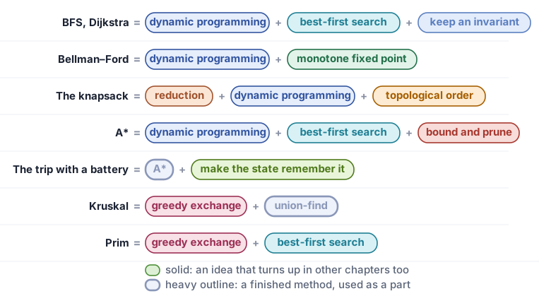
Breadth-first search and Dijkstra’s algorithm = dynamic programming + best-first search + keep an invariant. Dynamic programming: the search fills in Bellman’s equation from the smallest known cost upward. Best-first search: always take the most promising entry next, here the smallest known cost. Keep an invariant: every settled cost is final, and the queue holds what could still change. When every arrow costs one, a plain queue does the priority queue’s job, and the search is breadth-first search.
Bellman–Ford = dynamic programming + monotone fixed point. Dynamic programming: the cheapest cost with at most \(k\) arrows is built from the cheapest costs with at most \(k - 1\) arrows. Monotone fixed point: the costs only fall, so a round that lowers nothing has reached the answer.
The knapsack = reduction + dynamic programming + topological order. Reduction: a capacity and some items become a graph whose longest path is the best pick. Dynamic programming: the best pick is a longest path, so Bellman’s equation takes a maximum in place of the minimum. Topological order: the layers come one after another, so one pass fills them.
A* = dynamic programming + best-first search + bound and prune, on changed costs. A lower bound on the rest of the way gives every arrow a changed cost, and Dijkstra’s algorithm runs unchanged on the changed costs. So A* fills in Bellman’s equation by Dijkstra’s rule. Bound and prune: a vertex is never settled when its cost so far plus the bound is more than the goal’s cost.
The trip with a battery = A* + make the state remember it. Make the state remember it: when the battery’s charge decides what comes next, the charge goes into the state. A* then runs on the bigger graph unchanged.
Kruskal’s and Prim’s algorithms = greedy exchange. Greedy exchange: the cheapest link across a cut can be swapped into any minimum spanning tree, so taking it is safe. Kruskal’s algorithm adds union-find from the graphs chapter, to ask whether a link closes a cycle. Prim’s algorithm adds best-first search. Bellman’s equation still holds for the spanning tree, with the joined group as its state. After the big snow states that equation in words.
Every method of the main text but one runs the same search. The search takes a vertex and tries each arrow out of it. Whenever an arrow’s offer beats what the vertex at its end already has, the search keeps that offer. Kruskal’s algorithm is the one exception. Like Prim’s algorithm, it takes safe links, but in another order and with union-find. Outside the main text, Floyd–Warshall and the method by midpoints do not run this search either. They find the cheapest cost between every pair of vertices, and the section Other operations, the same equation shows both methods.
The methods that run this search differ in four choices.
- Which vertex comes next. What a method knows about the rest of the way decides this choice (Table 6.6). Dijkstra’s algorithm takes the vertex with the smallest known cost, and A* takes the vertex with the smallest known cost plus the estimate. Bellman–Ford takes every vertex again in rounds, and the method in topological order takes each vertex once.
- What an arrow offers. Usually it is the cost so far plus the arrow. In Prim’s algorithm it is the link alone.
- Which offer wins. Usually the smaller one wins. In the knapsack the larger one wins.
- What a state is. Usually it is a vertex of the given graph. With a battery it is a vertex with its charge, and in the knapsack it is a pair, how many items are decided and the weight used.
What lets each method choose as it does? Each one answers the chapter’s opening question by what it knows about the rest of the way (Table 6.6).
| What it knows about the rest of the way | The methods | So it can |
|---|---|---|
| only what it has worked out | Bellman–Ford | work the rest out exactly, in rounds |
| nothing in the rest leads back to a vertex already done | the method in topological order, the knapsack’s layers | decide each vertex once, in one pass |
| the rest costs \(\ge 0\) | Dijkstra’s algorithm | settle the smallest known cost at once |
| a lower bound on the rest | A* | aim the search at one goal |
| an exchange makes the rest irrelevant | Kruskal’s and Prim’s algorithms | take the cheapest safe link and never look back |
Faced with a new problem, ask which of the four choices it forces. Then, for each choice, ask what must be true for the proof to hold. The trip with a battery changes only what a state is. Its proof needs nothing new, because no arrow of the bigger graph costs less than 0. Transfer 1 asks the same two questions of the widest path.
Some of these parts can be swapped for another part that does the same job. Figure 6.27 shows a few, each beside the choice that this chapter made. The first four keep the promise. The last one breaks it. Prim’s algorithm with Dijkstra’s priority builds the tree of cheapest paths from one vertex. That tree does not always have the least total cost.
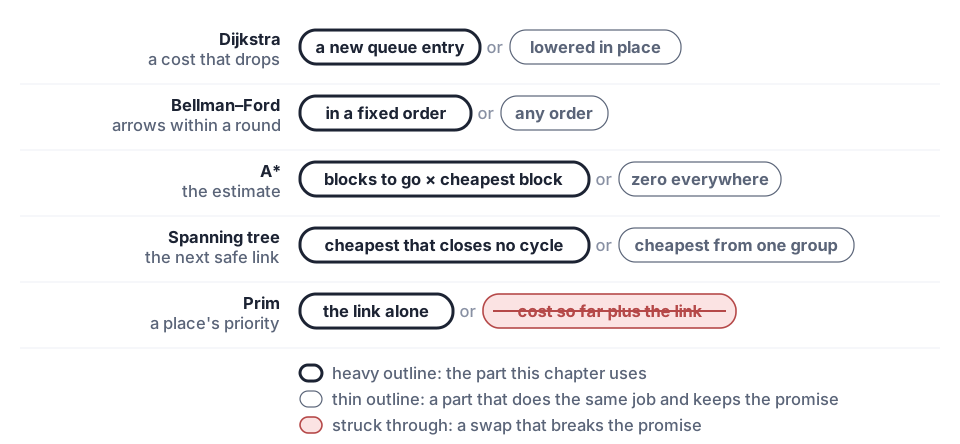
6.9.1 Choosing one, under pressure
| The question | The method | If its assumption breaks |
|---|---|---|
| fewest arrows to every vertex | breadth-first search | when costs differ, a path with more arrows can be cheaper |
| cheapest path to every vertex, no negative cost | Dijkstra’s algorithm | one negative arrow can leave a settled cost too high, with no warning |
| cheapest paths with negative costs | Bellman–Ford | none: a negative cycle is reported, not hidden |
| the best pick under a limit | the knapsack as a longest path | weights given as large numbers make the graph too big to build |
| cheapest path to one vertex, with a lower bound on the rest | A* | an estimate that drops by more than an arrow’s cost lets A* return a path that costs too much, with no warning |
| join everything at the least total cost | Kruskal’s or Prim’s algorithm | a cost that depends on who else is joined breaks the exchange, and greedy loses its guarantee |
6.9.2 What each one costs
| Method | Time | Space beside the graph | Measured |
|---|---|---|---|
| breadth-first search | \(\Theta(n + m)\) | \(\Theta(n)\) | 3.9 ms, New York, every arrow costing one |
| Dijkstra’s algorithm | \(O(m \log m)\) | \(O(n + m)\), a cost per vertex and the queue’s entries | 15 ms, New York |
| Bellman–Ford | \(O(nm)\) | \(\Theta(n)\) | 955 ms, New York, 614 rounds |
| in topological order | \(\Theta(n + m)\) | \(\Theta(n)\) | 2.6 ms, 100,000 vertices and 400,000 arrows, no cycle |
| the knapsack | \(\Theta(nC)\) for \(n\) items and capacity \(C\) | \(\Theta(nC)\), the layers | 187 ms, 1,000 items, capacity 100,000 |
| A* | \(O(m \log m)\), on the vertices it settles | \(O(n + m)\), a cost per vertex and the queue’s entries | 4.1 ms a trip, New York |
| Kruskal’s algorithm | \(O(m \log m)\), the sort | \(\Theta(n + m)\), the sorted links and union-find | 103 ms, a million vertices, two million links |
| Prim’s algorithm | \(O(m \log m)\) | \(O(n + m)\), a priority per vertex and the queue’s entries | 476 ms, the same graph |
6.9.3 The same ideas, over and over
| Idea | Where else it runs |
|---|---|
| best-first search | Dijkstra in OSPF; A* in route planners, on the navigation meshes of game engines and in the ROS 2 robot planners; the geometry chapter’s search for the nearest point |
| dynamic programming | git diff and DNA alignment, in the studio; GPS map matching in OSRM; the dynamic-programming knapsack solver of OR-Tools; Bellman–Ford’s rounds; the knapsack’s layers |
| monotone fixed point | RIP and Babel routing; chess endgame tables, worked back from the positions already won or lost until a round labels nothing new [33], [34, Sec. 12.1.9], pp. 543–544; the graphs chapter’s spreading inside a knot |
| reduction | knapsack as a longest path; currency arbitrage as a negative cycle |
| bound and prune | A*’s estimate; alpha-beta search in chess programs such as Stockfish [35, p. 10] |
| make the state remember it | charge in the state for electric routing; direction in the state for hybrid A* |
| greedy exchange | single-linkage clustering; image segmentation; the unrouted connections that KiCad draws on a circuit board; the first camera directions in COLMAP’s global mapper (Kruskal) [36]; the matroid theorem in the appendix |
How do route planners on road maps answer in milliseconds? They add one more idea, which is to do their slow work once, in advance. A contraction hierarchy ranks the vertices and adds shortcut arrows that skip the unimportant ones. Then every query searches only upwards in that ranking [37], and every answer stays exact. Learned estimates give up that guarantee for a better guess. DeepCubeA trains a network to estimate how far a Rubik’s cube is from solved, and it searches with that estimate [38]. Such an estimate is often good. But it is not a lower bound, so A*’s promise does not come with it.
Bellman’s equation is also used far beyond maps. In control, suppose the motion is linear. Suppose also that the cost of every step is a quadratic function of where the system is and of how hard it is pushed. Then the cost still to go is a quadratic too, and the controller for this setting is the linear-quadratic regulator. When Bellman’s equation runs backwards from the last step in this setting, it becomes the Riccati equation of control theory [39, pp. 149–151]. In continuous time, Bellman’s equation becomes the Hamilton–Jacobi–Bellman equation. Along the best path, the slope of the cost still to go is the costate of Pontryagin’s principle [39, pp. 109–110, 117]. Published work on the Formula 1 power unit, done with Ferrari and tested in simulation, uses the costate to spend the battery over a lap [40].
6.10 ◆ Where that leaves Sara big picture
By the end of the summer Sara could ride her deliveries without a map. By the spring she had taken one thing from the two seasons, a way to choose between the streets. When the cost of a street is never negative, the smallest known cost can be trusted at once. When a street can pay energy back, every street has to be tried again and again, until nothing changes. When she packs the box, she only needs to know how much room is left after each decision. When the address is far, she knows a time that no route can beat, and that time tells her which way to look. And in the snow, the shortest link out of the joined group was always safe, so nobody had to plan the whole lane first.
The chapter used story words for its first steps, and the usual words are these. A place is a vertex. A one-way street is an arrow, and a two-way one is a link. A route is a path, and the knapsack’s states are the vertices of a graph built for the question. A known cost is often called a tentative distance, and trying an arrow is relaxing it. A cheapest path is a shortest path, and a previous vertex is a predecessor. The estimate is A’s heuristic. An estimate that never overstates the rest is admissible, and one that keeps the box’s invariant is consistent*.
The summer’s question needed the rest of the way, as a cost to be worked out or as a bound to rely on in the search. The winter’s question could drop it, because an exchange made the rest irrelevant. Which kind will the next problem be?
6.11 ✎ Hands-on projects practice
The projects come first. In each one you build something, measure something, or explain something to another person. A project has no single right answer, so you judge your work by the checks that the project asks you to build. After the projects come the self-check problems. These are numbered exercises, and each comes with an answer you can check. When a project needs code, let an AI write it. The times given assume that the AI writes it. But three things are still your job when the AI helps. You say what the code must do. You build the check that shows the code does it. And you judge what comes back.
Project 1 · checking · medium · ~1 hour
Check cheapest paths you did not compute. Take a map of twenty vertices that has negative arrows but no negative cycle. Ask an AI for the cheapest cost of every vertex from one start, and for each vertex’s previous vertex. Before you ask, write down the checks that any right answer must pass.
- The start costs 0.
- For every arrow \(u \to w\) out of a vertex \(u\) with a cost, \(w\) has a cost too, and \(w\)’s cost is at most \(u\)’s cost plus that arrow.
- For every vertex \(v\) with a recorded previous vertex \(u\), there is an arrow from \(u\) to \(v\), and \(u\)’s cost plus that arrow is exactly \(v\)’s cost.
- Following the previous vertices back from every vertex with a cost reaches the start.
Say why these four checks are enough. Then delete one of them, and find a wrong answer that the weakened check lets through.
Project 2 · checking · medium · ~1 hour
Check a spanning tree. Ask an AI for a minimum spanning tree of a graph of thirty vertices. Write a check that needs no second tree for comparison. The answer must join everything and close no cycle, and every link left out must close a cycle when it is added. On that cycle, the left-out link must be the costliest, or tied for costliest. Say why this last check is the cut property read the other way. Then make two links cost the same, so that a second minimum tree exists, and say whether your check should pass it.
Project 3 · measuring · medium · ~1.5 hours
Where each method wins. Use a grid of 300 by 300 corners. First give every block the same time, and measure breadth-first search against Dijkstra’s algorithm. Then give the blocks random times, and measure Dijkstra’s algorithm against A* on the way to one far corner. Try three estimates for A: zero, the number of blocks still to go times the cheapest block’s time, and half of that. For each run, report the number of corners settled and the time taken. Say for which estimate A’s extra work stops saving time.
Project 4 · design · hard · ~3 hours
Design a trip planner with a battery, with an AI. A delivery bike has a battery of a fixed size. Each street in the town takes minutes and energy, and some streets give energy back on the way downhill. Some places have sockets that charge the battery at a fixed rate. The planner must give the quickest trip from one place to another that never runs the battery flat. The chapter’s methods give one answer to this. Find your own, and check that it keeps what it promises.
- Write the problem first. Write the top half of a box: goal, promise, cost and assumptions. Leave the idea and the invariants empty for now.
- Check the promise in the library’s Lean contract. Read
Workbench.Contractin the library’sWorkbench/Spec.lean. It is the contract that every planner must keep. It says what a trip is and when a battery runs flat. Check that each line says what your promise says. Where it does not, change your promise, or say why the contract is wrong. - Design the state. Say what a state of your graph is. Then say why two visits to the same corner with different charge must count as two different states.
- Choose the method and the estimate. Say whether any arrow of your graph costs less than 0 minutes, and what that lets you use. Give an estimate that keeps A*’s invariant.
- Build the check before the code. Write a slow planner that tries every trip that passes no state twice. Say why that is enough, and compare the two planners on small towns.
- Let an AI write the planner, and give it the bench,
algodesign.paths.workbenchinpython/algodesign/paths/workbench.py. The bench builds towns and runs a planner on trips it keeps hidden. It checks every answer against the contract and counts what the planner reads. A planner sees the town only through the bench’sTown, which counts every read. The functionjudgebuilds towns from the seeds that you give it and runs the planners on them. The plannerchapter_candidateis the chapter’s method. Runjudgeon seeds of your own, with your planner besidechapter_candidate. Then run your own checks, and judge what comes back.
Hand in the final box whole, with a line for each repair saying whether it fixed the code, the box or the design, and why. ★ Prove in Lean that your design meets Workbench.Contract.
Another brief or another AI would give another run, and this is one of them. The bench is the library’s algodesign.paths.workbench. It builds towns and runs a planner on trips that it keeps hidden. It checks every answer against Contract, and counts what the planner reads.
Round 1. We checked the promise against the three parts of Contract, and they matched one for one, so nothing changed. But the check showed two things that the box leaves unsaid. First, the contract reads “flat” as below empty, so a trip may arrive with nothing left. Second, it allows at most one street from one place to another. With that rule, a list of places names the streets of a trip. The AI made each state a place at one battery level, and it searched the states with Dijkstra’s algorithm. It skipped any state when the same place had already been settled at a level with at least as much battery, since more battery never makes a trip slower. It read each place’s streets once per trip and kept them until the trip ended. The planner passed on the hidden towns, and every answer kept the contract. Of its 48 answers, 20 had a charging stop and 12 said there was no trip. On the trip that needed the most reads, it read the town 39,233 times. The chapter’s Dijkstra on the states reads a place’s streets each time it settles a state there, so it made 3,722,806 reads on its costliest trip.
The AI’s note found two holes. First, the box never said whether a battery at exactly empty has run flat. The AI found out by trying both readings on the bench. The box should have given that answer. The check in step 2 had seen the gap, and still left the words as they were. Second, the count saw only the reads of the town. Why does that matter? A planner that keeps the streets can look at them again for free. This one went over a place’s streets again for every battery level it took there. A copy of the town recorded every look at a street, and on the trip with the most looks it counted 2,528,431 looks. The bench had counted 37,909 reads for the same trip, so that is about 67 looks for every read. Fix the box: a trip never takes the battery below empty, and it may arrive at empty. The cost counts every street and socket that the planner looks at during a trip, whether it reads them from the town or from anything that it keeps of the town. What the bench cannot count is checked by reading the code.
Round 2. A fresh AI got the mended box. Its planner keeps no streets, and it asks the town again each time it takes a state. Before each trip it searches back from the goal over the map with the battery left out. This search skips every street that takes more than a full battery. The quickest times to the goal found this way never claim too much, so they make a safe estimate. With it, A* heads for the goal and still returns the quickest trip. The same search marks the places that cannot reach the goal at all, so a start among them gets “none” at once. We asked which estimate never makes the search return a slower trip, and the AI named this one. The reason is that every real trip rides the map, and charging only adds minutes. The AI added two more conditions. Along every street, the estimate must drop by at most that street’s minutes, as A*’s box asks. And it must be the same at every battery level of a place. This planner also skips a state at a place already settled with at least as much battery, as the first round’s planner did. If either of the AI’s two conditions fails, that skip could lose the quickest trip. The planner passed on the hidden towns, and every answer kept the contract. It made 250,038 reads per trip on average, about a seventh of the chapter’s 1,832,084 reads. Its costliest trip took 1,885,727 reads, about half of what the chapter’s costliest trip took. A reading of the code found only one thing that the planner looks at without a count, a table of minutes to the goal. The planner builds that table on each trip, and its own box names the table. Nothing to repair.
Along the way the AI noted three things that no check catches. First, a trip given as a list of places cannot say which of two streets between the same two places it rides. The contract already asked for one street at most, and the towns had no such pair, but the box never said so. The final box says it now. Second, the bench counts memory only after the last trip, and by then a planner that lets go of everything holds nothing. So the AI measured its own peak inside a trip, which was 1,441,577 numbers. Third, consider a trip ruled out only because the battery runs down along the way, one street at a time. Such a trip would make the search go through every state that can reach the goal. The hidden towns held no such trip. Every trip with no answer had a goal that the map alone rules out. Each such goal was either a place to which no street leads, or a hilltop where every street leading in takes more than a full battery. So the bench never asked for a trip that only the battery rules out. The choice of towns is therefore part of the check.1
In 2020 a user of petgraph, a Rust graph library, reported that its A* returned a path that was not the cheapest [27]. Here is the graph from the report. The arrows A to B, B to C and C to D cost 3 each, A to C costs 8, and A to D costs 10. The goal is D. The estimates are 9 at A, 6 at B, and 0 at C and D.
- Before running anything, say whether each estimate is a lower bound on the cost still to go. Then say whether the estimates keep the box’s invariant along every arrow.
- Run A* by hand, settling each vertex once. Say what cost it returns for D, and what the cheapest cost really is.
- Say which line of the A* box the report’s estimates break. Then say what petgraph had to change so that it returns the cheapest path even with such estimates.
Only after you have your own answer, hand the graph and the estimates to an AI and ask what A returns. Does it actually run the steps, or does it recite what A is supposed to return?
6.12 ✎ Self-check problems practice
Transfer 1 · middling · ~25 min
The widest way. The cargo bike is wide, so Sara wants the route whose narrowest street is as wide as possible. The street widths, in decimeters, are A–B 3, A–C 5, B–D 4, C–B 4, C–D 2, D–E 4 and B–E 1. In graph words, each street is a link with a width. Change Dijkstra’s algorithm so that a vertex’s priority is the width of the narrowest link on its path so far, and the largest priority comes off first. Find the widest way from A to E. Then say which part of Dijkstra’s box this change touches. Which part of the promise still holds, and what takes the place of “no negative arrow”?
The widest way is A, C, B, D, E, and its narrowest street is 4 decimeters wide. The method settles A first. It then settles C at a width of 5 decimeters, through A–C. Next it settles B at a width of 4 decimeters, because going through C beats the 3 decimeters of the direct street. Then it settles D at a width of 4 decimeters, through B. Last it settles E at a width of 4 decimeters, through D, because B–E would give only 1 decimeter. The arrow’s offer changed, from “cost so far plus the arrow” to “the smaller of the width so far and the street’s width”. The winning offer changed from the smaller to the wider. So the choice of the next vertex changed too: the widest comes off first. The promise still holds. Each vertex gets the width of a widest way to it. The new Assumes is that a path never gets wider when it goes one link further. It takes the place of “no negative arrow”, which says that a path never gets cheaper when it goes one arrow further.
Transfer 2 · middling · ~30 min
At most one stop. Here are the flights from Home and their fares: to Vienna 100, to Munich 50, to Lisbon 320. Vienna to Lisbon costs 100, Vienna to Munich costs 10, Munich to Paris costs 50, and Paris to Lisbon costs 50. Sara’s aunt will fly with at most one stop. What is the cheapest fare to Lisbon with no stop, with at most one stop, and with any number of stops? Then look at Figure 6.9. Say whether the table or the one list answers “at most one stop”, and why the other cannot answer it.
With no stop the fare is 320. With at most one stop, which means at most two flights, the fare is 200 through Vienna. With any number of stops the fare is 150 through Munich and Paris. The table answers the question. Row \(k\) holds the cheapest fare with at most \(k\) arrows, and “at most one stop” is row 2. The one list that Bellman–Ford keeps cannot answer it, because the list can run ahead of its row. Suppose each round goes through the places in the order Home, Vienna, Munich, Lisbon, Paris. Then the list’s first round already gives Lisbon 150, which is a fare of three flights. So the list cannot tell you what two flights cost.
Transfer 3 · middling · ~30 min
Heights from Bellman–Ford. Take the three places and arrows of Figure 6.7: the Bakery to the Square costs 2, the Bakery to the Hilltop costs 4, and the Hilltop to the Square costs \(-3\). Add a new vertex with an arrow of cost 0 to each of the three places, and run Bellman–Ford from the new vertex. Use the costs it finds as heights. Then give each arrow \(u \to v\) a changed cost, its old cost plus the height of \(u\) minus the height of \(v\). Say whether any changed cost is negative. Run Dijkstra’s algorithm from the Bakery on the changed costs, and turn its costs back into energies.
Bellman–Ford from the new vertex gives the heights 0 for the Bakery, 0 for the Hilltop and \(-3\) for the Square. The changed costs are 5 (Bakery to Square), 4 (Bakery to Hilltop) and 0 (Hilltop to Square), so none is negative. Dijkstra’s algorithm gives the Square 4 and the Hilltop 4. To turn a cost back, take the changed cost, subtract the height of the path’s start, and add the height of the path’s end. The Square then costs \(4 - 0 + (-3) = 1\) and the Hilltop costs 4, and these are the right answers. This is Johnson’s method. It runs Bellman–Ford once, and then runs Dijkstra’s algorithm from every vertex.
Transfer 4 · middling · ~30 min
Every pair at once. There are four vertices. The arrows are 1 to 2 costing 3, 1 to 4 costing 7, 2 to 1 costing 8, 2 to 3 costing 2, 3 to 1 costing 5, 3 to 4 costing 1, and 4 to 1 costing 2. Fill the table of cheapest costs between every pair with Floyd–Warshall, updating one table in place. First allow vertex 1 in the middle of a path. Then allow vertices 1 and 2, and so on. Each time you allow a new middle vertex \(k\), set \(c(i, j) \leftarrow \min\big(c(i, j),\ c(i, k) + c(k, j)\big)\) for every pair \(i, j\). Then say what a number below zero on the table’s diagonal would mean, and why the method should stop there.
From 1: to 2 costs 3, to 3 costs 5, to 4 costs 6. From 2: to 1 costs 5, to 3 costs 2, to 4 costs 3. From 3: to 1 costs 3, to 2 costs 6, to 4 costs 1. From 4: to 1 costs 2, to 2 costs 5, to 3 costs 7. A diagonal entry below zero means there is a negative cycle through that vertex. Then no cheapest path exists between two vertices when a path between them can pass through the cycle, because each trip around the cycle lowers the cost again. The single table updated in place also breaks. Its entries stop meaning the cheapest cost over any set of middle vertices. An entry can fall much further than one trip around the cycle would lower it. So the method stops there and reports the cycle. Weiss explains why it is safe to update one table in place. Using a vertex as a middle vertex cannot improve a path that starts or ends at that vertex. But that reason holds only “unless there is a negative cycle” [4, p. 493].
Here are forty-one exercises. Each shows roughly how long it takes, and everything you need for them is in the chapter so far. The answers are on a page of their own.
If you only do four, do Exercises 2, 4, 13 and 16.
They are grouped by kind of task, not by method. To practice one method, here are the exercises for each section:
- The quickest way there: 1, 2, 3, 18, 26, 33
- Downhill pays: 4, 5, 6, 7, 19, 22, 28, 34
- What fits in the box?: 8, 9, 10, 20, 29, 35, 39
- What is this all about?: 11, 12, 23, 27
- Heading for the address: 13, 14, 15, 24, 30, 31, 37, 38, 41
- After the big snow: 16, 17, 21, 25, 32, 36, 40
6.12.1 Run it and report the state
Exercise 1 · gentle · ~10 min
Run breadth-first search from a on the graph of Figure 6.28. Every link can be taken both ways and counts one. Take each place’s links in alphabetical order of the place at the other end. The moment a place is found, give it its count and note the place that found it. In what order do the places come off the queue? How many links is each place from a, and what is each place’s previous vertex?
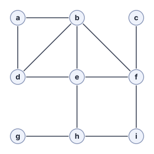
Exercise 2 · middling · ~20 min
Run Dijkstra’s algorithm from a on the graph of Figure 6.29, as the chapter’s code does. The number on an arrow is its cost, and a street drawn with two arrows has a cost each way. Try each settled place’s arrows in alphabetical order of where they lead. The queue hands out the smallest cost first. On a tie, the letter that comes first goes first. When a known cost drops, a new entry goes in. An offer equal to the known cost changes nothing. The old entry stays, and it is skipped when it comes off. In what order are the places settled, and at what cost? Which entries come off old and are skipped? What is each place’s previous vertex? Which cheapest path to i do the previous vertices give?
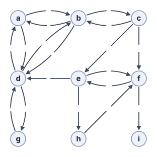
Exercise 3 · middling · ~15 min
The bread is sold at three counters: the Bakery, a kiosk at the Station and the School’s canteen. A customer who calls gets the loaf from the counter whose rider reaches the customer quickest by bike, in the minutes of Figure 6.3. Say what you would change in Dijkstra’s algorithm. Give every place’s time and its counter. Finally, say whether the box’s Assumes still holds.
Then: Now do the same another way. Add one new place, with an arrow costing 0 to each counter, and run Dijkstra’s algorithm unchanged from it. Which way changes the search, and which changes the map?
Exercise 4 · middling · ~20 min
Run Bellman–Ford from a on the graph of Figure 6.30, in place, as the chapter’s code does. Each round goes through the places in alphabetical order and tries each place’s arrows in alphabetical order of where they lead. Pass over a place that has no cost yet. A cost lowered early in a round is used later in the same round. Give the list after each round, until a round lowers nothing. How many rounds run, counting that last one? What is the cheapest path to f?
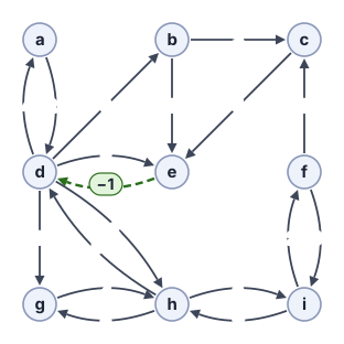
Then: Row 1 of the table holds the cheapest cost with at most one arrow. A place is ahead of row 1 when the list after round 1 gives it a cost where row 1 has none, or a lower cost than row 1. Which places are ahead after round 1, and why is that safe?
Exercise 5 · hard · ~25 min
The graph of Figure 6.31 has a negative cycle that a reaches. Run Bellman–Ford from a in place, as in Exercise 4, for six rounds, one per place. Which place does the sixth round lower last? From it, step back through the previous vertices six times: where do you land? Then keep stepping back until that place comes back. Which cycle is it? Write it reversed, so that each place is followed by the end of its arrow. What do its arrows total?
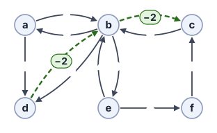
Exercise 6 · middling · ~20 min
A kitchen starts four dishes, a to d, at integer minutes \(x_a, \dots, x_d\), counted from a reference time, so a start may be negative. Each rule says one dish starts at most some minutes after another: \(x_b - x_a \le 5\), \(x_c - x_b \le 2\), \(x_a - x_c \le -4\), \(x_d - x_c \le 3\) and \(x_d - x_a \le 6\). Make a place for each dish, and one more place, s. Draw an arrow costing 0 from s to every dish. For each rule \(x_j - x_i \le c\), draw an arrow from \(i\) to \(j\) costing \(c\). Run Bellman–Ford from s and give each dish’s cost. Show that these costs, taken as start times, keep every rule. Then add the rule \(x_c - x_a \le 3\) and say why no start times can keep all the rules.
Exercise 7 · middling · ~20 min
A bank quotes: 1 euro buys 1.10 dollars, 1 dollar buys 0.90 euros, 1 dollar buys 150 yen and 1 yen buys 0.0062 euros. Make a place per currency and an arrow per quote. An arrow costs 1,000 times \(-\ln\) of its rate, rounded to an integer. Say why, before the rounding, a loop of trades that gains money is a negative cycle. Can the rounding change that? Then find such a loop with Bellman–Ford from the euro, and check that it really gains.
Exercise 8 · middling · ~20 min
A box holds 9 kilograms, and four orders wait: order 1 weighs 3 kilograms with a tip of 10, order 2 weighs 2 kilograms with a tip of 8, order 3 weighs 5 kilograms with a tip of 11 and order 4 weighs 2 kilograms with a tip of 4. Fill the knapsack’s layers one order at a time, as the chapter’s code does. From each state that some pick reaches, skip the order, or take it if it fits. At each weight, keep the larger gain. Then step back from the best state. If states tie, start from the one with the least weight. At each layer, take the order when taking it gives at least as much as skipping it. Give each layer as its weights and gains. Then give the best tips and the pick.
Then: The box now holds one kilogram more. What is the best pick now, and its tips?
Exercise 9 · middling · ~20 min
Turn the word lane into plant in as few edits as possible. Each edit inserts, deletes or changes one letter. As a graph, a state is a pair (i, j): i letters of lane used so far and j letters of plant used so far. The grid of Figure 6.32 has every state, with lane across the top and plant down the side. It has no arrows yet. Draw the three kinds of arrow out of a state. Across uses the next letter of lane alone and deletes it. Down uses the next letter of plant alone and inserts it. The diagonal uses one letter of each. What does each kind cost, and which arrows cost 0? Then give every state the cheapest cost of a path to it from (0, 0). Go a row at a time. Row j holds the states with j letters of plant used. How many edits does it take? There is only one cheapest path. Which edits does it make, and which letters does it keep?
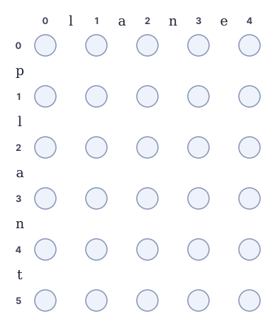
Then: git diff compares two files line by line, with inserts and deletes only and no change. Search this grid of letters the same way, with inserts and deletes only. How many edits does it take?
Exercise 10 · middling · ~20 min
Build the knapsack’s graph the other way around. A box holds 9 kilograms, and four orders wait: order 1 weighs 2 kilograms with a tip of 1, order 2 weighs 5 kilograms with a tip of 1, order 3 weighs 6 kilograms with a tip of 2 and order 4 weighs 3 kilograms with a tip of 3. Make a state a pair: how many orders are decided, and the total of the tips of the orders taken so far. From each state two arrows leave. One skips the next order and adds no weight. The other takes it, gains its tip and adds its weight, whether it fits or not. Fill the layers one order at a time, as in Exercise 8. This time, label each state with the lightest weight that a path into it carries. Give each layer as its tip totals, each with its lightest weight. Then read the last layer. What are the most tips whose lightest weight fits in the box? Which orders give them?
Then: How many states can a layer of this graph hold? For this box, how many can a layer of the graph of Exercise 8 hold? Which of the two graphs grows with the box’s size?
Exercise 11 · middling · ~15 min
The graph of Figure 6.33 has no cycle, and some arrows cost less than 0. Put it in Kahn’s order. Count the arrows into every place, and queue the places with none, in alphabetical order. Then, while the queue has a place, take the front place. Lower the count of each place at the end of its arrows, in alphabetical order, and queue a place when its count reaches 0. Now take the places in Kahn’s order, starting with a at cost 0. Pass over a place that no arrow has reached. For every other place, try each arrow out of it once. Give Kahn’s order, every place’s cost from a, and each previous vertex.
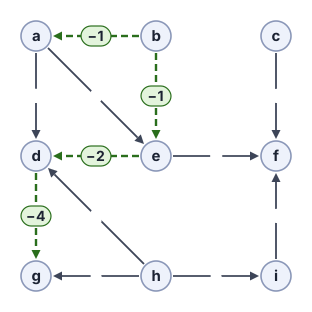
Exercise 12 · middling · ~15 min
On the graph of Exercise 2, work out the cost still to go to e from every place. This is Bellman’s equation read from the goal. Set \(r(e) = 0\). Then \(r(u) = \min_{u \to v} \big( \text{cost}(u \to v) + r(v) \big)\), as in equation (6.9). Next, start at a. At every place, take the arrow whose cost plus \(r\) at its end is smallest. On a tie, take the letter that comes first. Give \(r\) for every place, with none where e cannot be reached, and give the path.
Exercise 13 · hard · ~25 min
The graph of Figure 6.34 is a grid of corners. Each block can be ridden both ways, in the minutes it shows. No block takes less than 2 minutes. Run A* from f to j. The estimate is twice the number of blocks still to go, counted along the grid. Each entry’s priority is the known cost plus the estimate. The smallest priority comes off first. On a tie, the letter that comes first goes first. The search stops when j is settled. Which places are settled, in order, with their priorities? What does the path cost, and which path is it? With the same tie rule, how many places does Dijkstra’s algorithm settle, up to and including j?
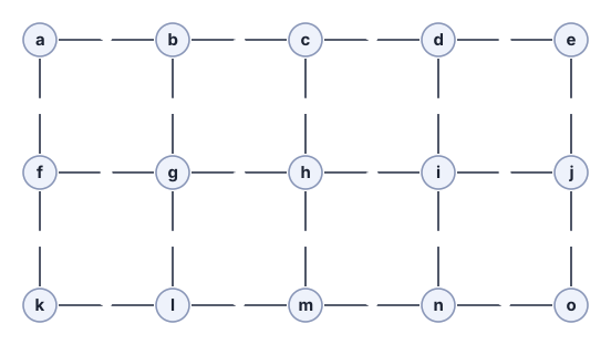
Exercise 14 · middling · ~15 min
On the graph of Figure 6.35, the number under each letter is an estimate of the cost still to go to f. Say whether each estimate is a lower bound on the cost still to go. Then say along which arrows the estimate drops by more than the arrow costs. Next, run A* from a to f, as in Exercise 13, settling each place once. What cost does it give f, and by which path? What is the cheapest cost, and by which path?
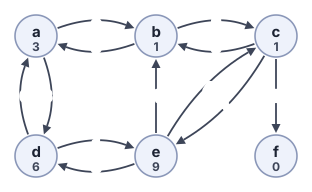
Exercise 15 · middling · ~15 min
A courier firm can send a van to the next town by three routes. Route A takes 20 minutes and has no toll. Route B takes 16 minutes and has a toll of 2 euros. Route C takes 10 minutes and has a toll of 3 euros. The firm pays at most 2 euros of toll a trip. Within that limit, it wants the quickest route. A planner turns the toll into minutes instead. At a price of p minutes for every euro, it picks the route with the smallest total of its minutes plus p times its toll. For every price of 0 or more, which route does it pick? Which route is quickest within the 2 euros? Is there a price that picks it?
Then: Suppose each road of a map has minutes and a toll. What must a state remember, so that a cheapest-path search finds the quickest route within the toll limit? Why can a price not do the same here?
Exercise 16 · middling · ~15 min
Run Kruskal’s algorithm on the graph of Figure 6.36. Take the links shortest first. Equal lengths go in alphabetical order of their ends, by the earlier end and then by the later one. Keep a link whose ends are not yet joined. Skip a link whose ends are joined already. Stop when one group is left. Which links does it look at, in order, and is each kept or skipped? Which links does it never look at, and what do the kept links total?
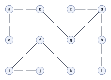
Then: Equal lengths now go the other way, latest letters first. Which links does the tree hold, and what does it total?
Exercise 17 · gentle · ~10 min
Run Prim’s algorithm on the graph of Exercise 16, starting at a. Keep taking the shortest link from a place already joined to a place not yet joined. Equal lengths go in alphabetical order of their ends, as in Exercise 16. In what order are the links added?
Then: Now give each place a priority equal to its cost from a so far plus the link, as Dijkstra’s algorithm does. Which links does the tree from a hold? How much longer is it than the cheapest tree?
6.12.2 Which promise broke
Each item hands you something that a program produced and claims to be correct. Say whether it is correct. If it is not, name the promise or invariant it breaks. If it is correct, saying so is the answer.
Exercise 18 · middling · ~10 min
A program computes the cheapest costs from a on the graph of Exercise 2 and returns a 0, b 8, c 9, d 4, e 15, f 17, g 10, h 16, i 18.
Exercise 19 · middling · ~10 min
Bellman–Ford, run from a on the graph of Exercise 4, reports the cycle d, g, h, d as a negative cycle.
Exercise 20 · middling · ~10 min
On the orders of Exercise 8, a program packs orders 1, 2 and 4, for 22 in tips. It says no pick that fits gains more.
Exercise 21 · middling · ~10 min
On the graph of Exercise 16, a program returns the links a–b, a–e, c–d, d–h, e–f, f–i, f–j, f–k, g–h, g–k, h–l, 29 in all, as a minimum spanning tree.
6.12.3 You supply the input
Exercise 22 · hard · ~20 min
Add one arrow to the graph of Exercise 2, out of i and costing −3. It must lead to another place, one to which i has no arrow yet. Choose it so that Dijkstra’s algorithm, run from a as in Exercise 2, gives some place a wrong cost while no cycle is negative. Give one that works.
Then: Name all the arrows that work, and say why the others do not work.
Exercise 23 · middling · ~15 min
Bellman–Ford on the graph of Exercise 4 takes the places in alphabetical order, and it needs several rounds. Give another order in which to take the places, so that the first round already gives every place its cheapest cost. Each place’s arrows are still tried in alphabetical order of where they lead.
Then: Say what every such order has in common.
Exercise 24 · hard · ~20 min
On the graph of Exercise 14, forget its estimates. Give a new estimate, one integer per place. It must keep the box’s invariant, and with it A* from a to f must settle only the places of the cheapest path.
Then: Say what every such estimate has in common.
Exercise 25 · middling · ~10 min
On the graph of Exercise 16, Kruskal’s algorithm leaves out b–f. Give b–f a new length, an integer of at least 1, so that Kruskal’s algorithm keeps it. Use the tie rule of Exercise 16.
Then: Name all the lengths that work, and say why.
6.12.4 Which idea do you reach for
Each of these exercises describes a situation, most of them far from maps. Which of the seven ideas from Table 6.9 would you use? Each exercise has four options. Pick the one you would reach for first.
Exercise 26 · gentle · ~5 min
A museum app tells a visitor at the entrance the walking time to every room. Corridors take different times, none negative. The app should show each room’s time as soon as it is certain, the nearest rooms first.
- reduction
- best-first search
- greedy exchange
- monotone fixed point
Exercise 27 · middling · ~10 min
A sawmill cuts a 12-meter log into pieces for sale. Its price list gives a price for a piece of each length from 1 to 12 meters, and a cut loses no wood. Which cuts bring the most money?
- greedy exchange
- make the state remember it
- dynamic programming
- best-first search
Exercise 28 · middling · ~10 min
A price site keeps the lowest price found so far for every product, in cents. A bundle’s price is built from the stored prices of the products in it. Every night the site goes through all the shops again, and the shops’ offers do not change during the night. A price it finds can only lower what is stored. When can it stop for the night?
- monotone fixed point
- dynamic programming
- best-first search
- greedy exchange
Exercise 29 · middling · ~10 min
A film festival has one screen and forty films, each with a start time, an end time and a rating. It wants screenings that never overlap, with the largest total rating.
- greedy exchange
- reduction
- best-first search
- make the state remember it
Exercise 30 · middling · ~10 min
A rail pass lets a traveler take at most three night trains and any number of day trains. A planner wants the cheapest trip between two cities that keeps to the pass.
- make the state remember it
- reduction
- monotone fixed point
- greedy exchange
Exercise 31 · middling · ~10 min
A puzzle app solves a sliding-tile puzzle in the fewest moves. A move slides one tile one square. From any position, the app can quickly add up how many squares each tile is from its home square. The app should look at as few positions as it can and still find the fewest moves.
- greedy exchange
- monotone fixed point
- bound and prune
- reduction
Exercise 32 · hard · ~15 min
A biologist has 500 samples and the distance between every two samples. The biologist wants them in 5 groups, so that the two closest samples in different groups are as far apart as possible.
- dynamic programming
- greedy exchange
- best-first search
- monotone fixed point
6.12.5 The tests pass. What did they miss?
Code that fails its tests is easy to catch. The costly kind passes every test, because nobody wrote a test for the requirement it breaks.
Exercise 33 · middling · ~15 min
A delivery app finds the quickest time from its depot to every address with Dijkstra’s algorithm. Its tests pass: on a thousand random maps, each in one piece, every time matches a slow search that tries every path. After launch, a bridge closes. The addresses beyond it show a time of 0 minutes, and drivers are sent there first. What requirement did the tests miss?
Then: Write the requirement as a sentence that a test could check.
Exercise 34 · middling · ~15 min
A currency desk finds the cheapest chain of exchanges from euros to every currency by Bellman–Ford. Each exchange is an arrow whose cost comes from \(-\ln\) of its rate, as in Exercise 7. Its tests pass: on random rate tables, every cost matches a slow search. Each test table is made from one price per currency, less a fee on each exchange. One morning the rates allow a loop of exchanges that euros can reach and that ends with more money than at its start. The desk prints its costs as on any other day. What requirement did the tests miss?
Then: Write the test.
Exercise 35 · middling · ~15 min
A warehouse packs a van with the knapsack as a longest path. Its tests pass: on random orders, the best value always matches a slow search through every pick. In use, the loaders find that the orders it lists weigh more than the van takes. What requirement did the tests miss?
Then: Write the test that would have caught it.
Exercise 36 · middling · ~15 min
A council plans which roads to clear after a storm with Kruskal’s algorithm, joining every village for the least work. Its tests pass: on random connected maps, the total always matches a slow search through every spanning tree. After a landslide splits the valley in two, the program stops with an error. It has read past the end of its list of roads. What requirement did the tests miss?
Then: Write the requirement as a sentence that a test could check.
6.12.6 Fill in the contract
No options this time. The workload below is not one of the chapter’s. The answer is not a name but a short answer to each of the six questions in the contracts chapter.
Exercise 37 · hard · ~40 min
A strategy game moves units over a map of a million tiles. Each tile takes some seconds to cross, never a negative number. Roads make some tiles quicker. When a player clicks, the unit must start moving within two milliseconds, along the quickest way to the target. Players notice a unit that takes a needlessly slow way. Buildings go up during play and can block tiles. Work out the parts of a contract for this workload, in the order that the contracts chapter uses. Give one or two sentences for each part.
Then: Suppose a building blocks the way while a unit is on it. Which part of your contract says what happens then? Why does the method alone not settle it?
6.12.7 Fix the code, the box, or the design?
Each item starts from code that an AI wrote from one of the chapter’s design boxes. The code did something that looks wrong. Decide which of three things happened. The code breaks a promise in the box: fix the code. The code keeps the box but misses what you wanted: fix the box. The design keeps its promise, but its assumptions or its cost no longer fit the job: change the design. Say why.
Exercise 38 · middling · ~10 min
An AI writes A* from its box for a courier firm. The estimate is 0 at every place, so the code is Dijkstra’s algorithm to one goal. Asked for the cheapest path from a to g on the graph of Exercise 2, it stops as soon as g is settled. To plan the next order, the dispatcher reads the cost of f off that answer, 17. But the cheapest path to f costs 16. Which of the three is it, and why?
Then: Rewrite the line of the box that has to change. Say what the change costs, and give the cost that the dispatcher expects.
Exercise 39 · middling · ~10 min
A shipping firm packs containers with the knapsack as a longest path, as the chapter builds it. For years it has weighed everything in kilograms. A new customer weighs in grams: 30 parcels and a container that takes 20 tonnes, so the container holds 20,000,000 grams. The code follows the chapter’s Python, and it is still correct. But a single packing now runs for minutes and fills gigabytes of memory. Which of the three is it, and why?
Then: Name a design that fits, and say what it costs.
Exercise 40 · middling · ~10 min
An AI writes Kruskal’s algorithm from the box, but it keeps one mark per place instead of union-find. A link is kept unless both its ends are marked already, and keeping a link marks its ends. On the graph of Exercise 16 it keeps 9 links, 23 in all. Which of the three is it, and why?
Then: Name a test you would keep from the AI.
6.12.8 The cheapest trip with one free arrow
Exercise 41 · hardest in the chapter · ~60 min
You already have:
- Dijkstra’s algorithm and its box, printed in the chapter
- the box’s Assumes, in its words, “No arrow costs less than 0”
- the charge in the state: a state of a new graph is a place together with what the trip still has left
A courier has one voucher, which makes one street of a trip free. No street costs less than 0. Write a procedure, as code or as precise steps, that finds the cheapest trip from one place to another. The voucher may be used at most once. Your answer must say what a state of your graph is. It must say which arrows leave each state, and what they cost. It must also say why the cheapest path in your graph is the cheapest trip with the voucher, and why Dijkstra’s algorithm may run on that graph.
Two checks tell you whether you got it right:
- On the graph of Figure 6.37, from a to i, your trip costs 7, with the voucher on a→d.
- The cheapest trip without the voucher costs 14. Making its costliest arrow free gives 8, more than 7.
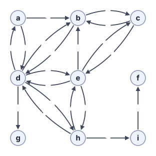
If a state of your graph is a place together with whether the voucher is used, the graph has twice as many states as the map has places, and three arrows for every arrow of the map. Another graph that gives the same costs is just as right, for example one with an extra goal state, or one that leaves out the states no trip reaches.
Stretch: Extend it to k vouchers. How does the work then grow with k and the arrows?
- Without the book, say why Dijkstra’s algorithm can settle the smallest known cost at once. Then say what one negative arrow does to that reason.
- Draw a map of three vertices where Dijkstra’s algorithm gives a wrong cost, even though no cycle is negative.
- Say why Bellman–Ford’s one list may run ahead of the table, and why that is safe.
- Turn three orders and a cargo box into the knapsack’s graph, and say what a path in it is.
- Give an estimate for A* on a grid, and say why it never claims too much.
- Say the cut property in one sentence, and say why it makes Kruskal’s choice safe.
- Pick one of the chapter’s design boxes and write it from memory: what it promises, its idea and invariants, and on what its cost depends. If it assumes anything, also say what you would see if that assumption broke. Then open the box and compare.
- Name the chapter’s methods in order. For each one, say what it knows about the rest of the way. Then say what it could not do, which forced the next method.
Whichever of these you could not reconstruct is the one to reread, and only that one. If you got all eight, come back again in a month instead.
6.13 ★ Frontier map advanced
What follows is optional. It is a short tour of ideas just past the edge of this chapter. Skip it now if you’d rather move on, and come back later.
The methods of this chapter are decades old, and they are still the ones that run. The entries below come in three kinds. Some are recent results that broke a bound that had stood for a long time. Some are limits that still stand, each in the model where it holds. The rest are places where the chapter’s ideas now run, most of them in AI and robotics. Each entry ends with a question you can now ask of any claimed improvement.
6.13.1 Dijkstra’s bound, broken and made optimal
Below the sorting barrier; instance optimality
Dijkstra’s algorithm hands out the vertices in order of cost. Keeping that order costs as much as sorting. But the question asks only for each vertex’s cost, not for the vertices in order of cost. In 2025 Duan, Mao, Mao, Shu and Yin looked at sparse directed graphs, which have few arrows per vertex. The arrow costs are real numbers \(\ge 0\), in a model where a method may only compare and add costs. For that case the five authors gave the first deterministic method that beats the sorting bound. The method mixes a few Bellman–Ford rounds into Dijkstra’s algorithm, so that fewer vertices wait in sorted order. On a graph of \(n\) vertices and \(m\) arrows it takes \(O(m \log^{2/3} n)\) time [41, pp. 1–2]. A year later four of the five authors lowered that to \(O(m\sqrt{\log n \log\log n})\) [42, p. 1].
A second result, by Haeupler, Hladík, Rozhoň, Tarjan and Tětek, is about methods that must list the order. Suppose Dijkstra’s algorithm gets a queue that is quick to hand out the entries inserted most recently. Then, on every fixed graph, it is as fast as any method that must list the vertices in order of cost, up to a constant factor [43, pp. 1, 3]. So the two results do not clash. The first wins by not listing the order. The second is, up to a constant factor, the best among methods that must list it. For a single trip, the authors of the second result also proved bidirectional search optimal in the number of arrows at which it looks. A slip in that proof was later found and repaired. On a graph with at most one link or arrow between two vertices, bidirectional search stays optimal only on links, not on one-way arrows. Even there, each vertex’s links must come in random order [44, pp. 1, 4–5], [45, p. 1], [46, p. 1].
A bound is not yet a program, though. A preprint reports that, on graphs of up to ten million vertices, Dijkstra’s algorithm ran 3 to 4 times faster than one implementation of the 2025 method [47, p. 1]. In programs, the speed comes from a faster queue instead of a new bound. SimdQuickHeap splits its entries around pivots, as quicksort does, and compares several entries with one instruction. It was the fastest queue on every graph that its authors tested [48, pp. 1, 15]. When does a better bound become a faster program?
6.13.2 Downhill, fast
Negative costs, faster than Bellman–Ford
Bellman–Ford pays \(O(nm)\) for the right to handle negative costs. Can we pay less? For integer costs that are never below \(-W\), Bernstein, Nanongkai and Wulff-Nilsen gave a randomized method whose time is \(O(m \log^8 n \log W)\), nearly linear in the arrows [49, p. 1]. Their main tool is the tilt. The paper calls the heights a price function. It notes that A*’s estimate, the heuristic, is also a price function [49, p. 7]. The hard part is finding the heights. The method finds them piece by piece, with Dijkstra’s algorithm as the inner search. A year later Bringmann, Cassis and Fischer cut “nearly six log-factors” [50, p. 1].
Real costs held out longer. Fineman’s method of 2024 was the first to beat \(O(mn)\), at about \(mn^{8/9}\) [51, p. 1]. In a preprint, Khanna and Song give a method that takes \(n^{2+o(1)}\). That is almost linear when nearly every pair of vertices is joined [52, pp. 1–2]. On a sparse map with real costs, none of these is near linear. Is Bellman–Ford’s bound the end, and for which costs?
6.13.3 What stays out of reach
Pseudo-polynomial knapsack; linear-time spanning trees
The knapsack’s time, \(\Theta(nC)\) for \(n\) items, grows with the capacity \(C\), and that size is a number written in the input. So the method is pseudo-polynomial [11, p. 271]. A method polynomial in the numbers’ digits is not expected, because Subset Sum is NP-complete [11, p. (8.23)], p. 492. What can still move is the exponent. For \(n\) items and a heaviest weight \(w_{\max}\), Jin’s 2024 method takes \(O(n + w_{\max}^2 \log^4 w_{\max})\) time. That matches a conditional lower bound up to small factors [53, p. 1]. The bound assumes that (min,+)-convolution needs about \(N^2\) steps for two lists \(a\) and \(b\) of \(N\) numbers each. Entry \(k\) of its result is the smallest sum \(a_i + b_j\) with \(i + j = k\). That problem is proved equivalent to variants of the knapsack [54, p. 1].
Kruskal’s algorithm spends most of its time sorting the links. Can a spanning tree be found in linear time? Chazelle called this “perhaps the oldest open problem in computer science”. His deterministic method takes \(O(m\,\alpha(m, n))\) time, where \(\alpha\) is the inverse of Ackermann’s fast-growing function [55, p. 1028]. Karger, Klein and Tarjan’s randomized method takes linear expected time [56, p. 321]. Pettie and Ramachandran gave a deterministic method that is provably the best possible. Yet “the exact function describing it is not known at present” [57, p. 16]. So the best deterministic method is known, and nobody knows exactly how fast it runs.
In practice the speed comes from parallel rounds. Borůvka’s method lets every group take its cheapest link at once. ECL-MST combines it with Kruskal’s algorithm on graphics cards. The fastest competing code took about 4.5 times as long as ECL-MST on average [58, p. 1]. The GPU library RAFT builds on ECL-MST [59]. Which of these limits is proved, and which only waits for a method nobody has found?
6.13.4 Work done before the question
Customizable route planning
The contraction hierarchy of the big-picture section does its slow work once, for one set of street costs. Customizable contraction hierarchies split that work in two. The first part ranks the vertices by how their streets meet. The second fills in the current costs. When traffic changes the costs, only the second part runs again. A 2025 survey finds the framework “competitive in performance to both Contraction Hierarchies (CH) and Customizable Route Planning (CRP)” [60, pp. 1, 4].
A second way keeps an old hierarchy for A*. Traffic only ever makes a street slower. So the exact costs on an empty road make an estimate that never claims too much [61, pp. 1, 9, 13]. Timetables take the same idea. A preprint reports that T-REX answers a trip across Europe’s trains and buses in less than 10 ms. T-REX is 20 times faster than the method on which it builds [62, p. 1]. Learned distance indexes are only approximate. On 13 road maps, the ten indexes tested were typically within 3% of the true cost [63, pp. 9–10]. What does a prepared answer cost when the map changes, and is it still exact?
6.13.5 A path through regions
Graphs of convex sets
A robot arm reaching into a shelf must make two choices. It must choose which way around each obstacle to go, and the exact motion along that way. Marcucci, Petersen, von Wrangel and Tedrake make both choices one cheapest-path problem. Convex regions cover the free space. Each region is a vertex, and overlapping regions are joined. The path picks a piece of trajectory inside every region it visits [64, pp. 3, 8]. Because the path must choose its regions and its points inside them at the same time, the problem is NP-hard [65, pp. 4–5]. Still, solving a relaxed version and rounding it usually lands close to the best. For a simulated quadrotor in 100 random buildings, the rounded trajectory’s cost was within 1% of the best trajectory’s cost in 95 of them [64, pp. 17–18].
There are catches, though. The regions must be found first, and the arm’s regions were seeded by hand [64, p. 19]. The relaxed version can also be arbitrarily loose [65, p. 11]. The fact under Bellman’s equation is that every piece of a cheapest path is itself a cheapest path. That fact fails here, because the best way into a region depends on the point where the path arrives [66, p. 3]. GCS* keeps the fact point by point and carries A* over. In its exact form it is optimal and complete [66, p. 1]. When one vertex of your graph stands for many states, is there still one cheapest cost to reach it?
6.13.6 The battery’s whole range
Energy-optimal profile search
Sara knew her charge when she left the Bakery. A planner that does not know the charge must answer for every starting charge at once, with the cheapest route in energy for each one. Ahmadi and Jalili compute that with an A* that keeps several labels per vertex instead of one cost. It settles each label once, as Dijkstra’s algorithm settles a vertex. It also drops any label that another one beats. On real road maps with energy won back downhill, it ran about as fast as A* for one known starting charge [67, p. 1]. Their maps almost never have a negative cycle, and the reason is the one that this chapter gave. “Due to the law of conservation of energy,” the paper says, “such graphs are typically free of negative cycles” [67, p. 1]. What does an answer for every starting value cost, against an answer for one?
6.13.7 Other operations, the same equation
The cost still to go in machines; all pairs; cost algebras
The sum of the next step and the rest of the way, equation (6.9), steers real machines. NASA’s rover Perseverance landed on Mars in February 2021, and its driving software ranks the paths it could drive next by this sum. The software uses Dijkstra’s algorithm to estimate the cheapest cost from each path’s end to the goal. It then adds that estimate to the path’s own cost [68, p. 2], [69, p. 1].
Reinforcement learning calls the cost still to go a value function. Value iteration applies equation (6.9) to every state, round after round, just as Bellman–Ford’s rounds try every arrow [70, Sec. 4.4], p. 83.
Control engineers split the cost in the same way, but after a few steps instead of after one. Model predictive control plans a fixed number of steps from the current state. It often adds an estimate of the cost still to go after those steps. It then uses only the first step, and it plans again once the next state is known [39, p. 366], [71, p. 93].
Floyd–Warshall finds the cheapest cost between every pair of vertices at once. It allows one more vertex in the middle of a path at a time, and its work is \(O(n^3)\) for \(n\) vertices. The method by midpoints builds paths of \(2k\) arrows from paths of \(k\) arrows, and its work is \(O(n^3 \log n)\). Both work only when the graph has no negative cycle. Transfer 4 runs Floyd–Warshall by hand.
Bellman’s equation uses a pair of operations. The first takes the smallest value over the arrows into a vertex. The second adds an arrow’s cost to the cost of the vertex where the arrow starts. Replace that pair with another pair of operations, and the same equation does other jobs. With the largest sum, it finds the knapsack’s longest path. With a sum of products, it counts the paths into a vertex in a graph with no cycle, when every arrow carries 1. With the largest product, it finds the likeliest path, when every arrow carries a probability. The starting values change with the pair. The start gets 0 when the second operation is a sum, and it gets 1 when the second operation is a product. Every other vertex starts at a value that the first operation always passes over: \(\infty\) for the smallest cost, \(-\infty\) for the largest sum, and 0 for a count or a probability. When the first operation picks a best value, as the smallest and the largest do, Edelkamp and Schrödl call the pair a cost algebra. They state Bellman’s equation over any cost algebra and carry Dijkstra’s algorithm and A* over to it [34, Sec. 2.3], pp. 76–78. Replacing the pair also turns Floyd–Warshall into a check that constraints agree [34, Sec. 13.2.3], p. 579. Which pair of operations does your problem need, and does it keep the order on which Dijkstra’s algorithm relies?
6.13.8 Three steps and a learned rest
Model predictive control with a learned value
A controller often cannot afford to plan all the way to the end. So such a controller plans a few steps and estimates the rest. TD-MPC2 learns that estimate together with a model of how the world responds. It plans 3 steps ahead and adds the learned value of the rest. Then it uses each plan as model predictive control does [72, pp. 3, 5, 27]. With one set of settings it improved on the compared methods across 104 control tasks [72, p. 1]. But should such an estimate claim too much or too little? Here control and search disagree. Stability proofs for model predictive control need one fact about the states near the goal. From each of them, some step must lower the added cost by at least that step’s own cost [71], Assumption 2.14, p. 114. An added cost like that never claims too little. A* asks for the other direction. Its estimate must never claim too much. TD-MPC2’s authors warn that handing control of physical robots to a learned model “can result in catastrophic failures if no additional safety checks are in place” [72, p. 9]. Should an estimate of the rest stay at or below the true cost, as A* needs, or at or above it, as a stable controller needs?
6.13.9 When the rest has no single value
Depth-limited search in games
A chess program works out a few moves exactly and estimates the rest. That is the same split that TD-MPC2 makes for a controller. An evaluation function values the position at the depth limit [73, p. 888]. AlphaZero learned its evaluation from games against itself. It looked at 80,000 positions a second where Stockfish looked at 70 million, and it still beat Stockfish. The reason is that its network also suggests which moves to search [35, pp. 2–3, 5]. Ruoss and colleagues went to the other end. A transformer trained on Stockfish’s move values uses no search at all, and it still plays at grandmaster level against people. It remains weaker than Stockfish [74, pp. 1, 9]. Poker breaks the split. With the cards hidden, “states do not have well-defined values” [75, p. 1]. So Brown, Sandholm and Amos let the opponent choose among several strategies for the rest of the game at the depth limit [75, p. 1]. Pluribus was built that way, and it beat elite professionals at six-player no-limit Texas hold’em [73, pp. 888–889]. Student of Games plays chess, Go, poker and Scotland Yard with one search guided by learned values [76, pp. 1, 12]. When does a position have one cost still to go, and who chooses the rest of the game?
6.13.10 The next step, or the whole at once
Decoding and diffusion
A language model writes an answer one word at a time. After each word it does not know the cost of everything that follows. So it runs a search with no estimate of the rest. Greedy decoding takes the likeliest word. Beam search is a breadth-first search that keeps only the best few partial answers at each depth. It drops the other partial answers by rank, before any bound has shown that they cannot lead to the best answer. That is why nothing like A*’s promise comes with it. Guided by a learned judge of partial answers, beam search did best at small budgets. With the same judge at large budgets, beam search fell behind the method that samples many whole answers [77, p. 9]. A model can still look ahead inside one step. When Claude 3.5 Haiku writes a rhyming couplet, it activates features for words that could end the next line, before it writes that line [78], sec. “Planning in Poems”. In theory, a model that thinks in vectors instead of words can hold many next steps at once. It holds “a superposition state that encodes multiple search frontiers simultaneously” [79, p. 1]. Diffusion models drop the word-by-word order. Diffuser “predicts all timesteps of a plan simultaneously” [80, p. 2]. LLaDA writes text the same way, starting from an answer with every word masked [81, p. 3]. Even there Bellman’s equation comes back. Read a diffusion model as optimal control, and the logarithms of its densities obey a Hamilton–Jacobi–Bellman equation, the continuous form of this chapter’s equation [82, p. 1]. When a system writes the whole answer at once, what plays the role of the cost still to go?
6.13.11 Machines that write the estimate
Language models as search designers
Language models now write parts of a search. In Thought of Search a model writes only how to step from one state to the next and how to recognize the goal. A plain breadth-first or depth-first search does the rest. On four planning problems this solved every task with a few calls to the model [83, p. 1]. Tree of Thoughts lets the model propose and rate partial solutions. On the Game of 24 it solved 74% of the tasks, where step-by-step prompting solved 4% [84, pp. 1–2]. But an estimate written by a model might simply be wrong. LeanPlan guards against that. Its model also writes a Lean proof that its estimate for A* is zero at the goal and drops along any step by at most the step’s cost. Lean’s kernel checks the proof before the planner may use the estimate. A preprint reports that LeanPlan solved 281 tasks from the 2023 planning competition, which is 27.1% more than the best earlier optimal planner solved [85, p. 2]. Training alone gives no such guarantee. A network trained never to claim too much can still do so [86, p. 1]. Training a model on recorded searches also teaches less than it seems. Searchformer was trained on A*’s searches, and it solved 93.7% of unseen Sokoban puzzles with a cheapest plan [87, p. 1]. Yet models trained on search steps copied from unrelated problems did about as well [88, p. 1]. Where no good estimate is found, search stops helping. The builders of DeepSeek-R1 dropped a tree search over the model’s own words, because “training a fine-grained value model is inherently difficult” [89, p. 64]. Who writes the estimate, and who checks that it keeps the box’s promise?
6.14 ★ Appendix: why the shortcuts are safe advanced
This appendix is part of the chapter. The chapter used five facts without proving them, and here we prove each one. The code for each is in the companion library, in its paths folder.
- The old entries in Dijkstra’s queue are safe and few.
- The tilt keeps every cheapest path, and Bellman–Ford can find its heights.
- Apart from ties, A* settles a set of vertices that can be named in advance.
- When every cycle has a positive cost, Bellman’s equation has the cheapest costs as its only answer.
- Taking the cheapest is safe on a matroid and can fail off one.
6.14.1 Why the old entries are safe and few
Dijkstra’s algorithm, as the library runs it, pushes a new entry whenever a known cost drops. It does not remove the old entry, which stays in the queue (Listing 6.2). The section Settling one place at a time said that the new entry comes off first. That leaves the proof one job: show that an old entry comes off only after its vertex is settled. The first of the two facts below does that job, and the second shows that the old entries are few.
Of a vertex’s entries, the first to come off carries its known cost, and every later one is skipped. When does a vertex get a new entry? Only when an arrow gives it its first cost, or a cost strictly below the one it has. That cost then becomes its known cost. So if we line up a vertex’s entries in the order they were pushed, their costs fall strictly, and the newest entry carries the known cost. Now take a vertex \(v\) at the moment when its first entry comes off. None of \(v\)’s entries has come off before, so the newest one is still in the queue. The queue always hands out its smallest entry. Of \(v\)’s entries the newest is the smallest, so the entry that comes off is the newest one, at \(v\)’s known cost. That is the cost at which \(v\) is settled. From then on no entry is pushed for \(v\), because the algorithm never tries an arrow into a settled vertex. Every other entry of \(v\) was pushed earlier, at a higher cost. Such an entry comes off later, finds \(v\) settled and is skipped. Skipping it loses nothing, because \(v\) already has a lower cost.
The queue never holds more entries than there are arrows, plus one. The start’s entry is the first. Every other entry is pushed while an arrow is tried, and one try pushes at most one entry. An arrow is tried only once its start is settled. A vertex is settled only once, so each arrow is tried at most once. In all, then, at most \(m + 1\) entries are pushed, for \(m\) arrows, and as many come off. A push or a pop on a binary heap of at most \(m + 1\) entries takes \(O(\log m)\) steps. So the queue’s work is \(O(m \log m)\), plus a step per vertex to set up. Why is this the same as \(O(m \log n)\)? With at most one arrow from each vertex to each other vertex, \(m < n^2\) for \(n\) vertices. Taking logarithms gives \(\log_2 m < 2 \log_2 n\), and the constant 2 disappears inside the \(O\).
A* keeps the same queue. It only raises each priority by the estimate at its vertex, which is a fixed number per vertex, so the order of a vertex’s own entries does not change. Both facts therefore hold for A* word for word. Prim’s algorithm works the same way. A vertex’s offers there also fall strictly, when we compare them as pairs of cost and link (Listing 6.12). Each link is offered at most once, from the first of its ends to join the tree. So Prim’s queue never holds more entries than there are links. That is the same bound as for the lazy form that offers every link that crosses from the tree [90], Prop. M, p. 618.
6.14.2 Back to Dijkstra’s speed: the tilt
Sara’s town hides a way back to Dijkstra’s speed. An arrow’s energy is its distance plus the height it climbs. Take the height change away again, and every arrow costs its distance, which is never negative. Does that change which path is cheapest? No. Along any path, the height changes add up to the height at its end minus the height at its start. So taking them away moves only the total. It moves by the same amount for every path between the same two places, so the cheapest path in distance is the cheapest in energy too. The same move works on any graph. Give every arrow a changed cost: its cost plus the height at its start minus the height at its end. A* made the same move, with minus the estimate as each vertex’s height. With the right height for every vertex, the changed costs turn a map with negative arrows into one that Dijkstra’s algorithm can handle. Figure 6.38 shows it as a tilt of the town. The heights can even be found by running Bellman–Ford once. That is Johnson’s method, below and in Transfer 3.
What about a cycle? A cycle starts and ends at the same vertex, so its changed costs add and subtract the same height. The cycle’s total in changed costs is therefore its own total. So no choice of heights removes a negative cycle. In particular, on a map with a negative cycle, no heights make every arrow at least 0. To see why, suppose some heights make every arrow at least 0. Then the cycle’s total in changed costs is at least 0. But that total is the cycle’s own total, which is negative [1], Lemma 23.1, p. 663.
When no cycle is negative, Bellman–Ford finds heights that work. Give each arrow \(u \to v\) the changed cost \(\text{cost}(u \to v) + h(u) - h(v)\), as Transfer 3 does. Add a new vertex \(q\) with an arrow of cost 0 to every vertex, and run Bellman–Ford from \(q\). Does the new vertex create new cycles? No. Arrows only leave \(q\), and a cycle through \(q\) would need an arrow into it. So every cycle lies in the old map, and Bellman–Ford reports a negative cycle exactly when the old map has one. If it reports none, let \(h(v)\) be the cheapest cost from \(q\) to \(v\). This is a number for every vertex, since \(q\) reaches them all. Now take any arrow \(u \to v\). A cheapest path to \(u\) followed by the arrow is a path to \(v\), and \(h(v)\) is at most the cost of any path to \(v\). So \(h(v) \le h(u) + \text{cost}(u \to v)\), which says exactly that the arrow’s changed cost is at least 0. This is Johnson’s method [1, p. 664].
6.14.3 Which vertices A* settles
Write \(d(v)\) for the cheapest cost from the start to \(v\), \(r(v)\) for the cheapest cost from \(v\) to the goal \(t\), and \(h\) for an estimate that keeps the box’s invariant. The same search, on changed costs showed that A* settles the goal at \(d(t)\). Two more facts follow from the invariant.
The estimate never claims too much. Take a cheapest path from \(v\) to the goal, \(v = v_0, v_1, \ldots, v_k = t\). The invariant says that along each of its arrows the estimate drops by at most the arrow’s cost, \(h(v_i) - h(v_{i+1}) \le \text{cost}(v_i \to v_{i+1})\). Add these inequalities up. On the left every middle estimate appears once with a plus and once with a minus, so they cancel, and \(h(v) - h(t)\) is left. On the right the arrow costs add up to the path’s cost, \(r(v)\). So \(h(v) - h(t) \le r(v)\). Since \(h(t) = 0\), the estimate is never more than the rest of the way, \(h(v) \le r(v)\). In the usual words, a consistent estimate is admissible [19, Sec. 3.5.2].
Before the goal, A* settles every vertex with \(d(v) + h(v) < d(t)\), and no vertex with \(d(v) + h(v) > d(t)\). We first show that the priorities that come off the queue never fall. When a vertex \(u\) is settled, its priority is \(d(u) + h(u)\), its settled cost plus its estimate. Every entry that \(u\) pushes is for an arrow \(u \to w\), with priority \(d(u) + \text{cost}(u \to w) + h(w)\). That priority is at least \(d(u) + h(u)\), because the invariant gives \(h(u) - h(w) \le \text{cost}(u \to w)\). \(u\) came off with the smallest priority in the queue, so every entry still waiting has a priority of at least \(d(u) + h(u)\). So neither the new entries nor the old ones can bring a smaller priority later. Now look at the goal. It comes off with priority \(d(t) + h(t) = d(t)\). Every vertex settled before it came off with a priority of at most \(d(t)\), since priorities never fall, and that priority is \(d(v) + h(v)\). So no vertex with \(d(v) + h(v) > d(t)\) is settled before the goal. That is the second half.
For the first half, take \(v\) with \(d(v) + h(v) < d(t)\). Suppose, for a contradiction, that the goal comes off while \(v\) is still unsettled. On a cheapest path from the start to \(v\), let \(x\) be the first vertex not yet settled. Every vertex before \(x\) on that path is settled, and the path up to \(x\) is a cheapest path to \(x\), because part of a cheapest path is itself cheapest. A* keeps invariant 2 of Dijkstra’s box on the changed costs. By that invariant, \(x\)’s known cost is at most \(d(x)\). It cannot be lower, since every known cost is the cost of a real path, so it is exactly \(d(x)\). Its newest entry therefore has priority \(d(x) + h(x)\). Along the rest of the path, from \(x\) to \(v\), the estimate drops by at most what the rest costs, so \(h(x) \le d(v) - d(x) + h(v)\). Adding \(d(x)\) to both sides shows that \(x\)’s priority is at most \(d(v) + h(v)\). By the choice of \(v\), that sum is below \(d(t)\). So that entry would come off before the goal’s entry. This contradicts the goal coming off first, and so \(v\) is settled before the goal.
When no arrow is negative, an estimate of zero keeps the box’s invariant, and A* with it is Dijkstra’s algorithm. Applied to that case, the theorem says that Dijkstra’s algorithm, stopped at the goal, settles every vertex with \(d(v) < d(t)\) and none with \(d(v) > d(t)\). An estimate is never below zero, so a vertex that A* settles before the goal has \(d(v) \le d(v) + h(v) \le d(t)\). Apart from ties, then, A* settles only vertices that Dijkstra’s algorithm settles. The ties are why the comparison in the chapter needs a rule for ties [21], Thm 4.1. Check this on the grid across the river, where the address costs 16 minutes. Seven corners have a cost plus estimate below 16 minutes and three have exactly 16 minutes, and these ten are the corners that A* settled (Figure 6.19). The corner two blocks north of the bridge is 4 minutes out with 14 minutes estimated. Its cost plus estimate is 4 + 14 = 18 minutes. That is above 16 minutes, so A* never settles it.
6.14.4 When Bellman’s equation has one answer
What is this all about? called every method up to the knapsack an order for solving one equation. Why does the order not matter? When every cycle has a positive cost, the equation has only one solution. So whatever order a method uses, a list that solves the equation is the answer.
If every cycle has a positive cost, the cheapest costs are the only solution of Bellman’s equation. A solution gives the start 0 and every other vertex a number, or “unreachable”, which counts as more than every number. A minimum over no arrows is unreachable. Write \(d(v)\) for the cheapest cost to \(v\) and \(x\) for any solution. The proof has three steps.
The cheapest costs solve it. First, a cheapest path to every reached vertex exists. Why? Cutting a cycle out of a path never makes it costlier, so we only need to look at paths that pass no vertex twice, and there are only finitely many of them. Next, take any arrow \(u \to v\). A cheapest path to \(u\) followed by the arrow is a path to \(v\), so \(d(v) \le d(u) + \text{cost}(u \to v)\). The last arrow of a cheapest path to \(v\) gives equality, because the path up to that arrow is a cheapest path to the vertex where the arrow starts. So \(d(v)\) is the minimum over its arrows, and the cheapest costs solve the equation.
Every solution \(x\) has \(x(v) \le d(v)\) for every vertex \(v\). Take a cheapest path from the start to \(v\), \(v_0, v_1, \ldots, v_k\). Each vertex after the start takes the minimum over its arrows, and the minimum is at most the sum for any one arrow, so \(x(v_{i+1}) \le x(v_i) + \text{cost}(v_i \to v_{i+1})\). Start from \(x(v_0) = 0\) and go arrow by arrow. Each step adds at most the arrow’s cost, so at the end \(x(v) \le d(v)\).
Every solution \(x\) has \(x(v) \ge d(v)\) for every vertex \(v\). Take a vertex \(v\) other than the start whose \(x(v)\) is a number. Its minimum is reached by some arrow \(u \to v\), with \(x(v) = x(u) + \text{cost}(u \to v)\). Then \(x(u)\) is a number too, since otherwise the sum would be unreachable. Step back from \(v\) to \(u\), then back along the arrow that gives \(x(u)\), and so on [11, p. (6.27)], p. 296. Only two things can happen. If the steps reach the start, they trace a path whose arrows add up to \(x(v) - 0\). So \(x(v)\) is the cost of a real path to \(v\), and \(d(v)\) is at most the cost of every real path to \(v\). This gives \(x(v) \ge d(v)\). If the steps never reach the start, some vertex comes back, since there are only finitely many vertices. Between its two visits the steps go round a cycle on which every arrow is used with equality. Add up these equalities round that cycle. Every \(x\) appears once on each side and cancels, so the cycle costs exactly 0. But every cycle has a positive cost, so this case cannot happen. So every vertex with a number is reached from the start. A vertex that no path reaches therefore has \(x\) unreachable too, the same as its \(d\). Together the second and third steps give \(x = d\) [31], Thm 3.2, p. 67.
Does Sara’s town meet the condition? Yes. Every cycle of her town has a positive cost in energy, because its climbs and drops cancel and its distance is left. A cycle of cost exactly 0 breaks the theorem, and a tiny example shows how. Take an arrow of cost 1 from the start to \(a\), and arrows of cost 0 from \(a\) to \(b\) and back. Then \(x(a) = x(b) = s\) solves the equation for every number \(s \le 1\), because \(a\) takes the smaller of 1 and \(s\), and \(b\) takes \(s\) from \(a\). Only \(s = 1\) is the cheapest cost. The second step still holds on such a map, so \(x \le d\) for every solution \(x\). So the cheapest costs \(d\) form the largest solution. Bellman–Ford finds them anyway, because every cost that it holds is the cost of a real path (Why the rounds are safe), and no real path to \(a\) or \(b\) costs less than 1.
6.14.5 Why taking the cheapest is safe on a matroid
Formally, a matroid is a set of elements, here the links of a graph, with a family of subsets called independent, here the sets of links that close no cycle. A subset that is not independent is called dependent. Two rules make it a matroid. First, a subset of an independent set is independent. Second, if one independent set is smaller than another, some element of the larger can be added to the smaller, and the result is still independent.
Why do links obey the second rule? Call the smaller set \(A\) and the larger set \(B\). The links of \(A\) close no cycle, and they split the graph’s vertices into groups. Each group is joined by the links of \(A\) inside it, and a vertex that no link of \(A\) touches is a group of its own. Inside a group of \(g\) vertices at most \(g - 1\) links fit without a cycle, and \(A\) has exactly \(g - 1\) links there, since its links join the group into one piece without a cycle. Count the links of \(B\) that lie inside groups of \(A\). There are at most as many of them as \(A\) has links. \(B\) has more links than \(A\), so at least one link of \(B\) runs between two groups of \(A\). Adding that link to \(A\) joins the two groups without closing a cycle.
Two consequences come first. Call an independent set maximal when no element can join it. First, all maximal sets have the same size. Suppose one maximal set has fewer elements than another. Then the second rule lets an element of the larger set join the smaller one, so the smaller set was not maximal after all. Second, the greedy choice below ends with a maximal set. Why? When greedy cannot add an element \(e\), its set plus \(e\) is dependent. Call that set \(D\). Greedy’s set only grows, so at every later moment greedy’s set plus \(e\) contains \(D\). By the first rule a set that contains a dependent set is dependent, so the element can never be added later.
On every matroid, taking the cheapest element that keeps the set independent, again and again, gives an independent set of the largest size with the least total cost [31], Thm 6.1, p. 276. The proof is the cut property in general form. Let the greedy choices be \(g_1, g_2, \ldots, g_k\) in order. By the consequences above they form a set of the largest size. Among the independent sets of the largest size, take the cheapest ones. Of these, take one, \(B\), that agrees with greedy for as long as possible. So \(B\) holds \(g_1\) to \(g_{i-1}\), and \(g_i\) is the first greedy choice that \(B\) does not hold, if there is one. Suppose first that \(B\) holds all \(k\) choices. Then it holds the greedy set. When one of two sets of the same size holds the other, the two sets are equal, so the greedy set is \(B\) and is cheapest. Otherwise \(B\) does not hold \(g_i\), and we derive a contradiction. Start from \(\{g_1, \ldots, g_i\}\), which is independent, because greedy built it. Use the second rule to keep adding elements of \(B\) until the set is as large as \(B\). The result is \(B\) with one element \(b\) swapped for \(g_i\), and \(b\) is not among the first \(i - 1\) choices, since those are in the result already. When greedy chose \(g_i\), the element \(b\) was available too, since \(g_1, \ldots, g_{i-1}\) and \(b\) all lie in \(B\), and a subset of \(B\) is independent by the first rule. Greedy took the cheapest available element, so \(g_i\) costs at most what \(b\) costs. So the swapped set costs at most what \(B\) costs. It has the size of \(B\), so it is one of the cheapest sets of that size too, and it holds \(g_1\) to \(g_i\). That contradicts the choice of \(B\).
Off a matroid the greedy choice can lose. Take a box of 10 kilograms and three orders, one of 6 kilograms with a tip of 12 and two of 5 kilograms with a tip of 7 each. Call a set of orders a pick when it fits in the box. The picks keep the first rule, since part of a pick that fits also fits. They break the second rule. The pick of the 6-kilogram order alone holds one order, and the pick of both 5-kilogram orders holds two. Yet neither 5-kilogram order fits beside the 6-kilogram order, because each such pair weighs 11 kilograms. Now watch greedy fail. Greedy takes the largest tip first, so it takes the 6-kilogram order with its tip of 12. Then nothing else fits. The two 5-kilogram orders together give 14 in tips.
In general, when the theorem is turned around to take the largest value first, it holds on every matroid whose values are never negative. Its converse holds too. Whenever the second rule fails, as here, some values make greedy lose [31], Thm 6.1, p. 276. Thursday’s orders keep both rules, and largest tip first finds the 18 in tips. Ines’s rule failed for a different reason. It ranked the orders by tip per kilogram, which is a different greedy choice.
Kruskal’s algorithm is this theorem on the graph’s links. Prim’s algorithm does not fit the theorem, because the links that it may take depend on the group it has already grown. Its sets come from a weaker structure, a greedoid [91, p. 93]. The cut property covers both.
_dijkstra_multisource.” networkx/algorithms/shortest_paths/weighted.py, lines 856–879, commit e59d718, https://github.com/networkx/networkx/blob/e59d71890e745effb3724dc4b5620b23f92e0ee3/networkx/algorithms/shortest_paths/weighted.py#L856-L879; accessed 6 November 2026, 2026.dijkstra.” src/algo/dijkstra.rs, lines 181–211, release 0.8.3, https://github.com/petgraph/petgraph/blob/[email protected]/src/algo/dijkstra.rs#L181-L211; accessed 6 November 2026, 2026.dijkstra_shortest_paths.” include/boost/graph/dijkstra_shortest_paths.hpp, lines 57–63, 145–155 and 380–387, commit e62d023, https://github.com/boostorg/graph/blob/e62d023c0bef25b748f4b3d8a5af0e4769bfa627/include/boost/graph/dijkstra_shortest_paths.hpp#L380-L387; accessed 6 November 2026, 2026.src/graph/bellman_ford.md, commit ebd43c8, 2026.--diff-algorithm.” Git documentation, https://github.com/git/git/blob/master/Documentation/diff-algorithm-option.adoc, commit ffffb98, 2025.hybrid_a_star.cc in the open-space planner, commit 075a74b, 2026.rotation_averaging.cc, commit 9371f7b, 2026.The rounds and numbers come from one run of the Python bench. The run used the hidden seeds 101, 202 and 303 in both families. Each town had about 10,000 places. A full battery was at level 100, and the bench asked for 8 trips in each town. The peak memory is the AI’s own, from the practice seeds 1, 2 and 3. A fresh AI wrote each round. It was given only that round’s brief and the bench’s interface. The second round also got the judge’s report on the first. The interface’s own description says how the towns choose the goals of trips with no answer. The briefs, the candidates and the script that judges them are in
scripts/design_run_paths/in the book’s repository.↩︎