4 Geometry and high-dimensional search
Space is a doubt: I must constantly mark it, designate it.
Georges Perec, Espèces d’espaces (1974)
4.1 Pharmacy, open now
Mia has just moved from Lisbon to Zagreb with her son, for a job she wanted, in a city she does not know yet. Everything here still has to be worked out from nothing. She cannot read the street names without stopping, she does not know which tram goes where, and every corner is a guess. At home she never had to think about where things were. Here the space itself is the problem.
On their first night in the new flat, at eleven, her son has a fever. The medicine she packed is somewhere in a box she cannot find. She picks up her phone and types pharmacy, open now, and five pharmacies appear on the map before her thumb has left the screen.
Here nearest means spatially nearest. A pharmacy that is almost the closest is a longer walk, at night, with a sick child, through streets she has never seen. And an answer that comes late is no answer. She is not going to stand in the hallway waiting for a map to think.
Look at what the phone just did. The service behind it holds every place on a continent, and at this moment millions of people are asking it something, each from a different spot. So nothing can be sorted in advance. Which pharmacy is nearest depends on where you stand, and everyone is standing somewhere else. Two pharmacies were closer to Mia than some of the five, and the phone left them out, because they were closed.
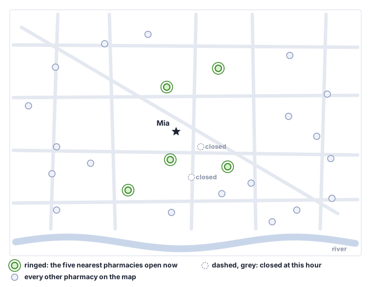
The plain way to answer her is to measure the distance to every pharmacy and keep the nearest. This is a linear scan, the search chapter’s sequential scan with a distance in place of a key comparison. It is exact, it needs no preparation, and every faster method in this chapter is checked against its answer, as the contracts chapter checked a clever method against the obvious algorithm as the definition. The chapter then prepares the map once, so that most places never need measuring at all, first for everything inside a strip of the map, then for the single nearest place. A month on, Mia will ask her phone something harder, a place like one she loved in Lisbon, and every idea that worked on the map will be tried again, in a space where it no longer works so well.
Start with the plain way, on a small example. Mia stands at \(q = (5, 5)\) on a grid. Six pharmacies are open around her, named by letters in the order they are stored: a \((2, 7)\), b \((6, 3)\), c \((9, 8)\), d \((4, 1)\), e \((7, 6)\) and f \((1, 4)\). Measure each one. The distance from \(q\) to a point \((x, y)\) is \(\sqrt{(x - 5)^2 + (y - 5)^2}\), but there is no need for the square root, because comparing squared distances picks the same pharmacy, and with whole-number coordinates they stay whole numbers.
\[ d^2\big((x, y), q\big) = (x - 5)^2 + (y - 5)^2 \]
For a, that is \(3^2 + 2^2 = 13\). The rest are b 5, c 25, d 17, e 5 and f 17. The nearest is b, at 5, and it is tied with e. A tie needs a rule, and the rule every structure in this chapter keeps is that the lower letter wins, the place stored first. So the answer is b, and the three nearest are b, e and a. Why the squares are always safe to compare, and what else near can mean, come later in the chapter.
Here is that scan in code.
None for no places.sq_dist adds up the squared differences, coordinate by coordinate, and enumerate hands over each place with its number, counting from 0, so a is 0, b is 1, and so on. A place keeps its number however a structure rearranges the places. For the \(k\) nearest, the library keeps the \(k\) best so far with the worst of them always on top, so each new place is compared with that one only (scan.py).
The scan measures every place, for every question. With \(n\) places, each question costs \(n\) distances, and nothing is learned between questions. The next person, standing a street away, starts again from scratch, and so does Mia if she walks to the corner and asks again.
Draw twelve points anywhere on squared paper. People ask from different spots, “which point is nearest me?”, millions of times. Design something you could prepare once that answers faster than measuring every point.
Five minutes. You’re done when you can name one point your design would never measure for some question, and say why it is safe not to.
Go back to the six pharmacies, and look at what each of the scan’s measurements told it. The distance to c says that c is 25 away, and it says nothing about any other pharmacy. That is the waste this chapter goes after. Every structure in it is a way to make one measurement tell you about more than one place. One comparison can rule out half a street. One distance can prove a whole region of the map too far away to matter.
4.2 Everything between two streets
Range tree
The next morning the fever is down, and the boy is asleep. Mia opens the map again, this time without hurry. She wants to know every pharmacy between her street and the river, the stretch she will walk every day, to the school and to work. That is not one place but a strip of the map, and the question is everything in it.
The keys 3, 9, 12, 17, 21, 26, 30, 41 are distances along a street. Report every key in the range from 10 to 28, ends included, while looking at as few keys as you can.
Five minutes, with a pencil. You’re done when you can say where the looking starts and stops, and name the keys you reported without looking at them one by one.
Did you start with the search chapter’s binary search for 10? It finds where 10 would go, between 9 and 12, one end of the range. Then you probably read 12, 17, 21 and 26 one at a time, until 30 told you to stop. Search for 28 as well, and follow both searches down a tree together. They go the same way until the two ends part. What lies between their paths after that?
4.2.1 Keys in the leaves
The search chapter’s ordered trees could already read off every key in a range, one at a time. This one hands a range back as a few whole subtrees, so that each can carry its own tree on the other coordinate. The tree keeps the keys at the bottom, in its leaves, sorted left to right. Every node above them is an inner node. It covers a run of the sorted keys, sends the first half to its left and the rest to its right, and holds the largest key on its left. When the count is odd, the left side takes the extra key, so the left half has \(\lceil n/2 \rceil\) keys. The key a node holds is then its lower median, and it separates the node’s two sides, as invariant 1 asks.
Build it on the eight keys from the exercise. The root covers all eight, sends 3, 9, 12, 17 left and 21, 26, 30, 41 right, and holds 17. Its left child splits 3, 9 from 12, 17 and holds 9. Its right child splits 21, 26 from 30, 41 and holds 26. One level further down, the nodes hold 3, 12, 21 and 30, and below each of them hang two leaves. The tree is three levels deep, since halving eight keys three times leaves one.
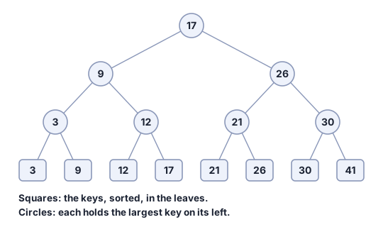
In code, the tree is built over positions in the sorted list rather than over the keys themselves. A leaf is one position, and an inner node covers a run of positions, from start up to just before end.
The constructor sorts the keys once, each with the number it was stored under, so the answer can name the stored places. The ... it leaves out refuses a key that cannot be ordered and keeps those numbers. build then never compares two keys at all, because the sorted list already says where every split falls. The whole class is in range_tree.py.
4.2.2 Where the two ends part
A query asks for every key from lo to hi. It starts at the root and walks down while the whole range lies on one side of the node’s key, going left when hi is smaller than the key and right when lo is larger. The first node where neither holds is where the two ends part. It is called the split node, and from there the walk becomes two walks [1, Sec. 5.1].
Below the split node, each walk follows the rules of Table 4.1. A subtree that lies wholly on the inner side of a walk is reported whole, without reading a key.
| walk | at a node with key \(s\) | then |
|---|---|---|
| to the split node | hi \(< s\) |
go left |
\(s <\) lo |
go right | |
| neither | stop: this is the split node | |
lo’s, from the split node’s left child |
lo \(\le s\) |
report the right subtree whole, go left |
\(s <\) lo |
go right | |
hi’s, from the split node’s right child |
\(s \le\) hi |
report the left subtree whole, go right |
hi \(< s\) |
go left |
Run it on the range from 10 to 28. The root’s key, 17, lies inside the range, so the root is already the split node. lo’s walk starts at 9, and 9 is smaller than 10, so it goes right, to 12. There \(10 \le 12\), so the whole right child, the leaf 17, is reported, and the walk goes left to the leaf 12, which is checked and is inside. hi’s walk starts at 26, and \(26 \le 28\), so the whole left child, 21 and 26, is reported, and the walk goes right, to 30. There 28 is smaller than 30, so it goes left, to the leaf 30, which is checked and is outside. The answer is 12, 17, 21 and 26.
Count what was read. Of the two leaves checked against the range, 12 went in and 30 did not. The leaves 17, 21 and 26 came out in whole pieces and were never compared with anything. The leaves 3, 9 and 41 were never reached at all.
Now a range that sits inside one subtree, from 18 to 25. At the root, 17 is smaller than 18, so the walk goes right. At 26, 25 is smaller than 26, so it goes left. At 21, the range lies on both sides, so 21 is the split node. Its left child is the leaf 21, checked and inside. Its right child is the leaf 26, checked and outside. The answer is 21. The walk down to the split node is the part a binary search would also do. What happens after it is what the tree adds.
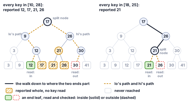
In code, the query collects the pieces, the canonical subtrees. They are whole subtrees, and the single leaves at the ends of the walks that passed their check.
The test not w.split < lo is how the code writes lo \(\le\) w.split, using only “smaller than”, so the same code works for any keys that can be ordered: numbers, words, dates. The ... returns nothing at once for an empty tree, or for a range whose lo is above its hi.
Walk it yourself below. Type a range, and before each step, say which way the walk goes.
Each walk goes down one level per step, and invariant 2 keeps the tree at most \(\lceil \log_2 n \rceil\) levels deep, since every level halves the keys. So a query costs two walks of at most \(\lceil \log_2 n \rceil\) steps, plus one step for each key it reports.1 For a million keys, that is about forty steps of walking, whatever the range, plus the answer itself.
Start above the split node. The walk went right only at a node whose key was smaller than lo. By invariant 1, nothing on that node’s left is larger than its key, so everything it left behind there is smaller than lo, outside the range. In the same way, it went left only past keys larger than hi. So every key in the range sits below the split node.
Below it, take lo’s walk. hi’s is the mirror. Every key on the split node’s left is at most the split node’s key, which is at most hi, so on this side only lo can rule a key out. At a node whose key is at least lo, the right child’s keys are at least that key (invariant 1), so they are all in range, and reporting them whole is right. At a node whose key is smaller than lo, the left child’s keys are no larger, so they are all out, and skipping them is right. Either way, the part the walk does not enter is decided, and the walk goes on into the part that is not. At the bottom one leaf remains, and it is checked on its own. So no key in range is missed.
Nothing is reported twice, either. Each reported piece hangs off the walk at a different node, so no piece lies inside another. The leaves at the ends of the walks sit on the walks themselves, not inside any piece.
4.2.3 Two coordinates at once
A strip on a real map is often a rectangle, between two streets running one way and two running the other. A list sorted by the first coordinate finds everything between the first pair of streets at once, but then every one of those places has to be checked on the second coordinate, and that can be nearly all of them. The tree does better, because the answer for the first coordinate is a few whole subtrees. Hang on every inner node a second tree of the same points, sorted by the other coordinate. A rectangle query reports the points inside both ranges. It walks the first tree as a range query on the first coordinate. In each whole subtree that walk would report, it runs a second range query on that subtree’s own tree, for the other coordinate, and reports what that finds. That is \(O(\log^2 n + k)\) time for \(k\) points reported, and \(O(n \log n)\) memory, since each point appears in one second tree on every level above it [1, Sec. 5.3]. The library’s two-coordinate tree is RangeTree2D.
4.2.4 What a strip can’t tell you
At eleven at night Mia did not want every pharmacy in a strip. She wanted the nearest one. A strip cannot answer that. Draw a square around her and it may be empty, or hold forty points. Even when it holds some, the nearest point can lie outside it. A point just past the middle of one side is closer than a point tucked into a corner inside. Widening the strip until something appears is guesswork. The nearest place needs a structure built for that question.
4.3 The nearest one, now
k-d tree
A strip can’t find the nearest pharmacy, and on the first night that was all Mia needed. One pharmacy, the closest. The scan finds it by measuring every pharmacy in the city, for every one of the millions of people asking. The k-d tree finds it by measuring about four.
Here are twelve points: a \((19, 8)\), b \((16, 4)\), c \((5, 17)\), d \((13, 18)\), e \((0, 10)\), f \((2, 19)\), g \((7, 16)\), h \((10, 2)\), i \((20, 20)\), j \((12, 0)\), k \((15, 11)\), l \((18, 7)\). Cut them in turns, first by x, then by y, then by x again. At each cut, sort that region’s points along the axis and split them in half. When the count is odd, the left side takes the extra point. The cut goes through the left side’s last point. Stop when every point is alone. Then stand at \((1, 13)\). Which regions must you open to be sure which point is nearest, and which can you leave closed?
Ten minutes. You’re done when you can name a region you never opened and say why leaving it closed was safe.
When you left a region closed, you compared two things. One of them was a distance to a point you had already measured. What was the other one, and where on the paper could you see it?
4.3.1 Cutting by turns
A map has two dimensions. Two numbers say where a place is, how far east and how far north. The range tree sorted along one of them. The k-d tree cuts the map itself into regions⬢, using both, in turns [1, Sec. 5.2], [2]. Cutting space into regions like this is a spatial partition. Each cut is a line straight across one region, along one axis, through the region’s lower median on that axis, just as each range-tree node split its keys. On one side of a cut, every point is at most the cut. On the other, every point is at least it (invariant 1). Each side gets half the points, and the left side takes the extra point when the count is odd (invariant 2). Then each side is cut along the other axis, and so on, until every region holds one point.
Here are the twelve points from the exercise. Sorted by x, the sixth point is j, at 12, so the first cut is \(x \le 12\), and e, f, c, g, h and j go left, the other six right. The left six, sorted by y, are cut at \(y \le 10\), below which sit j, h and e. The right six are cut at \(y \le 8\), below which sit b, l and a. The third round cuts by x again, at \(x \le 10\) and \(x \le 5\) on the left, \(x \le 18\) and \(x \le 15\) on the right. Each of those leaves a pair and a single point, and four more cuts by y, \(y \le 2\), \(y \le 17\), \(y \le 4\) and \(y \le 11\), split the four pairs. Eleven cuts, twelve regions of one point each, four levels deep. The build itself finishes each left side, down to single points, before it starts the right, and Figure 4.5 and the widget below number the cuts in that order.
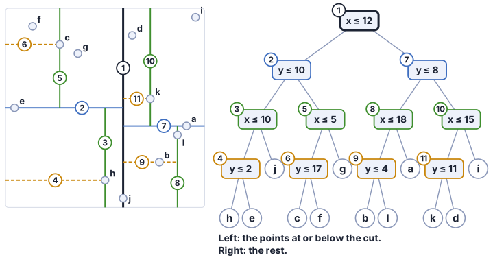
In code, the build is handed one list per axis, each holding the region’s points sorted along that axis.
order.by_axis[a] lists the region’s points, by their numbers, in order along axis a, and depth % self.dim takes the axes in turns. goes_left is a set of the left side’s points, so each split asks “is this point on the left?” once per point per list. Splitting a list this way never reorders it, which is why no region is ever sorted again, and the whole build costs \(O(n \log n)\) after the first sorts. The rest of the class is in kdtree.py.
Press Next step to build the tree one cut at a time. Before each press, say which axis the next cut uses and which point it goes through.
The same tree answers the rectangle question from the last section. Keep track of the rectangle each region covers. A region that lies wholly inside the query’s rectangle is reported whole, without looking at its points. A region that misses it is skipped. Any other region is opened, and its two sides are asked the same question (KDTree.range). On a plane it opens \(O(\sqrt{n} + k)\) regions for \(k\) points reported [1, Sec. 5.2], while the nearest search below can open all \(2n - 1\) regions, the leaves included, in the worst case.
4.3.2 The most promising region first
Now stand at \(q = (1, 13)\). The simplest search goes down to your own region, measures its point, and comes back up, crossing a cut only if the circle around you, as wide as the best distance so far, reaches past it. That is the depth-first search, and it works [3]. But the region it opens first is the one you stand in, which is not always the one that holds the answer.
A region is a box on the map. For each axis, the search below keeps an offset, how far \(q\) is from the box along that axis, or 0 if \(q\) lies between the box’s two sides on that axis. The sum of the squared offsets is the region’s bound, the least squared distance anything inside that region could have from \(q\). It is the squared distance from \(q\) to the nearest point of the box, and the search gets it from the cuts. Crossing a cut changes one offset only. On the far side, the offset along the cut’s axis becomes the distance from \(q\) to the cut.
\[ \text{bound} = \text{offset}_x^2 + \text{offset}_y^2 \;\le\; d^2(p, q) \quad \text{for every point } p \text{ in the region} \]
The search the library runs keeps every region it has not opened yet in a queue, each with its bound. A queue that always hands out the entry with the smallest key first is a priority queue. The scan’s keeper of the \(k\) best was one too, with the worst on top, and in code both are heaps. The search takes the region with the smallest bound, opens it, and puts its two sides back into the queue with their own bounds. When the region at the front of the queue is farther away than the best point found so far, everything still waiting is farther too, and the search stops. This is best-first search⬢, which opens the most promising region first [4].
How many points does the search have to measure before it can be sure of the nearest? Here is the search, step by step. The whole map has bound 0. Opening it puts the left half, e, f, c, g, h, j, in the queue at bound 0, since \(q\) stands in it, and the right half at \((12 - 1)^2 = 121\). The search opens the left half, then c, f, g, then c, f, then c alone, every one at bound 0, and measures c, at squared distance 32: \((5-1)^2 + (17-13)^2 = 16 + 16\). That is the best so far. But the queue still holds the region below the cut \(y \le 10\), with e, h and j, at bound \((10 - 13)^2 = 9\). Nine is less than 32, so a point in that region could still be nearer than c.
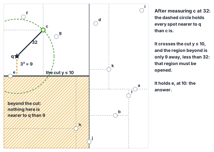
So it opens e, h, j, then e, h, then e alone, each at bound 9, and measures e, at 10: \((0-1)^2 + (10-13)^2\). Now the front of the queue holds g and f, each at bound 16, which is more than 10, and the search stops. Still waiting: g and f at 16, j at 90, h at 121, and the whole right half, six points, at 121. The nearest is e.
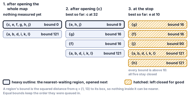
Count it. The search opened eight regions and measured two points, c and e. The other ten were never measured. And the first point it measured, c, was not the answer. The search found something good early, and the bounds told it exactly how far to keep looking.
A region stays closed only when its bound is already farther than the best point found⬢. Nothing in it can be closer, so skipping it keeps invariant 3. The code does it in a single line.
Two queues run side by side, one for the regions, nearest bound first, and one for the \(k\) best points, farthest first, so the point to beat is always on top. This function sits behind k_nearest_with_stats, in kdtree.py. The stop is strict. A region whose bound equals the \(k\)-th best distance is still opened, because a point in it at that same distance, stored earlier, would win the tie.
Play with it below. Drag \(q\) around the map, and before each step, say which region opens next. Then name every region that will still be waiting when the search stops.
Five minutes. You’re done when you have called three openings in a row before pressing the button, and named the waiting regions at the stop.
The appendix at the end of the chapter proves that leaving a region closed is safe. The same loop returns later in this chapter, walking a graph.
4.3.3 A map of who is nearest
There is a way to answer every question with no search at all. Give every spot on the map to the point nearest to it. The spots that belong to one point form a region around it, a cell, and the cells tile the whole map. This is the Voronoi diagram of the points, and the problem it solves has an old name, the post office problem. Which post office is nearest to this house [1, Ch. 7]? Store the diagram, and a question is one lookup. Which cell is \(q\) in?
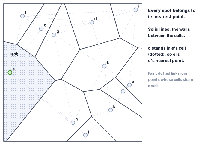
In the figure, a point’s cell shares a wall with only a few others, its neighbors, and they lie in different directions around it. The graph index in the second half of the chapter comes back to that picture.
4.3.4 How fast, measured
The box promised about four points measured, out of a million. Here is the run behind that. On one thread, the library built a k-d tree over 1,000,000 points spread uniformly over a square, with one point per leaf. Asked 10,000 nearest-neighbor questions, it answered about 830,000 questions a second, measuring 3.93 points per question on average, in a tree 20 levels deep, and each search opened about 30 of the tree’s regions.
The build can also stop cutting once a region holds 8 points or fewer, so each leaf keeps up to 8, and opening a leaf measures all of them. That runs faster still. The Python printed above cuts down to one point per leaf, as traced in this section.
On the same data, 8 points to a leaf answered 23% more questions a second. The tree is smaller, with about an eighth of the nodes, so a search takes fewer queue steps, and the points of a leaf sit together in memory. That more than pays for measuring about 14 points per question instead of four. On a million points in 20 tight clusters, each spread about 0.01 around a random center in the same square, the speedup was 34%. On the uniform points, the run’s peak memory, the points included, fell to under a third.
4.3.5 What the trick relies on
The circle around you, out to the best point found so far, crosses only a few of the tree’s cuts, the lines that split the map into regions. Most regions sit wholly outside it, and their bounds say so. That is a fact about two dimensions, and about any points that really spread in only a few directions, the low real dimension the box’s Assumes line asks for. A month from now, Mia’s question will put that assumption to the test.
4.4 The part of town she knows
Convex hull
Two weeks on, Mia knows a few places in Zagreb by heart: home, the pharmacy, the school, the café on the corner where the waiter now nods at her. She marks them on the map, and stretches a line around them. Inside that line is the part of the city she knows. Perec’s doubt, from the chapter’s opening line, has a border now.
Eight points: a \((1, 5)\), b \((4, 11)\), c \((10, 4)\), d \((0, 7)\), e \((8, 6)\), f \((3, 1)\), g \((9, 12)\), h \((12, 8)\). Stretch a rubber band around all of them. State a rule that decides, for any point, whether the band bends at it.
Five minutes. You’re done when your rule decides every one of the eight, including a, and you can say how many checks it costs for \(n\) points.
Your rule probably looked at pairs of points and asked whether all the others lie on one side of the line through them. That works. There is a faster way, and it builds the fence as you walk. Go left to right and keep the fence below the points seen so far. A new point can push the fence out. Which kept point does it leave inside, no longer a corner?
The rubber band is the convex hull of the points, the smallest fence with no dents that holds them all. It promises that every point is inside the fence or on it, and that the fence turns only at points. A point on a straight stretch of it is left out.
The algorithm rests on one question asked of three points. Walking from \(p\) to \(q\) and on to \(r\), do you turn left or right⬢? The answer is the sign of one number, the orientation of the three points:
\[ \operatorname{orient}(p, q, r) = (q_x - p_x)(r_y - p_y) - (q_y - p_y)(r_x - p_x) \]
It is positive for a left turn, negative for a right turn, and zero when the three lie on one line. So its sign says which side of the line from \(p\) to \(q\) the point \(r\) lies on.
Andrew’s monotone chain [5] builds the fence in two halves. Sort the points left to right, so the chain only ever moves right. Walk them in that order, building the lower half of the fence, and keep each new point. But first, while the last two kept points and the new one do not turn strictly left, drop the middle one, which cannot be a corner. Then walk right to left in the same way for the upper half, and join the two. At every moment, what is kept turns left at every point, which is what a fence with no dents does, walked counterclockwise [1, Sec. 1.1].
Run it on the eight points. Sorted left to right, they come as d, a, f, b, e, g, c, h. On the lower half, a is dropped as soon as f arrives, because d, a and f lie on one line, \(\operatorname{orient}(\mathbf{d}, \mathbf{a}, \mathbf{f}) = 0\), and that is not a strict left turn. Then b is dropped when e arrives, and when c arrives, first g is dropped and then e. The lower half is d, f, c, h.
Now walk the upper half yourself, back from h, and join the two halves.
Walking back from h, c is dropped when g arrives, e when b arrives, f when a arrives, and a when d arrives, so the upper half is h, g, b, d. Joined, without repeating the shared ends, the fence is d, f, c, h, g, b, counterclockwise from the leftmost point. a lies on the stretch from d to f and is left out. e is inside.
check_point turns each point into an (x, y) pair, and refuses one that has the wrong number of coordinates or a coordinate that is not a finite number. Sorting by (pts[i], i) puts equal points side by side in the order they were stored, so distinct keeps the first of each. The module is hull.py.
The slow rule from the exercise costs about \(n^3\) checks, every pair against every other point. Andrew’s method costs \(O(n \log n)\), and all of that is sorting the points left to right. Then it walks the sorted points twice, left to right for the fence’s lower edge, then back from the right for the upper. Each walk keeps every point once and drops it at most once. One new point can drop many, but each drop is paid for by the step that kept that point, the search chapter’s pay in installments, so the two walks together take steps proportional to \(n\).
Computed with ordinary floating-point numbers, the orientation of three nearly collinear points can come out with the wrong sign, and the fence gets a dent. The library’s orient2d computes the sign exactly, and the appendix shows a case where rounding lies.
4.5 What is this all about?
Nearest-neighbor and range queries
Step back from strips, cuts and queues for a moment. Under the scan, the range tree and the k-d tree, Mia has been asking two questions about a fixed set of places.
- Everything in this region. Every stored point inside a strip or a rectangle, a range query.
- The nearest one to here, or the \(k\) nearest, a nearest-neighbor query.
A delivery app asks which couriers are within reach of a restaurant, and which one is nearest. A game asks, many times a second, which players are close enough to see each other. A hospital asks which earlier scans look most like a new one. And a month from now, Mia will ask her phone for a café like the one she left in Lisbon.
4.5.1 What “near” is allowed to mean
Distances and similarity
Ranking needs only an order, and squaring keeps the order of distances, so no structure here takes a square root. Whole-number coordinates then give whole-number squared distances, and nothing is rounded at the comparison that decides the answer.
In the second half, a place is a long list of numbers, and two places are alike when their lists point the same way. Length is left out on purpose. A short note and a long review that say the same thing point the same way, at different lengths. The cosine of the angle \(\theta\) between two lists measures how alike they are, 1 when they point the same way. It needs no index of its own. Scale every list to length 1 once, when it is stored, and then
\[ d^2(u, v) = 2 - 2\cos\theta . \]
The nearest by squared distance is the most alike by cosine, so every structure built for distance answers the cosine question unchanged.
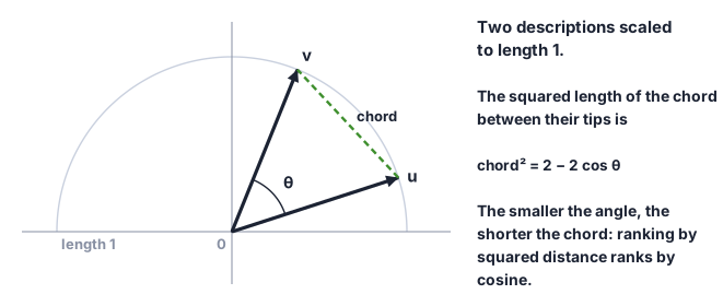
Under either meaning, the right answer is the scan’s, the stored point nearest by that measure, and the one stored first on a tie. Every approximate structure in the second half is measured against it.
4.5.2 What has been bought so far
Table 4.2 is the ledger for \(n\) points on a map.
| structure | prepare | one question | memory | which questions |
|---|---|---|---|---|
| Scan | nothing | every point | the points | nearest, \(k\) nearest, ranges |
| Range tree | sort once | two walks of \(\log_2 n\) steps, plus one step per point reported | about two nodes per point, and \(n \log_2 n\) with two coordinates | strips, and rectangles with two coordinates |
| k-d tree | sort once per axis | a few dozen regions, and 3.93 points measured per question, at a million uniform points | about two nodes per point | nearest, \(k\) nearest, rectangles |
What a structure saves in one column, it costs in another. The scan costs nothing to prepare, and the most on every question. The trees cost one build, and then each question measures almost nothing. On a map, the k-d tree’s row is very good.
Say Zagreb has a thousand cafés. Describe each with ten numbers you choose: price, noise, coffee, plants, opening hours, and so on. Two cafés are “near” when their numbers are. Does the k-d tree’s trick still work? Does a ball around your best café so far, the map’s circle with more numbers, still cross only a few cuts? With five hundred numbers?
Five minutes. You’re done when you can say what the ball crosses at ten numbers, and guess what happens at five hundred.
The eternal silence of these infinite spaces frightens me.
Blaise Pascal, Pensées (1670), no. 206 (Brunschvicg), trans. W. F. Trotter
4.6 A place like this one
The curse of dimensionality
4.6.1 From a map to a list of numbers
Two months on, the boy is fine, and Mia knows the way to work, to the school and to the pharmacy without looking. What she misses now has a shape. In Lisbon there was a small café two streets from her flat: quiet, strong coffee, plants on every sill, cheap, open late. She doesn’t want the nearest café. She wants that one, here.
On the first night the phone knew exactly what to do. “Nearest” is a question about the map, and the map knows where every place is. “Like hers” is a question about what a place is like, and the map knows nothing about that. So describe every place with numbers: price, noise, how strong the coffee is, how many plants, how late it closes. Ten numbers picked by hand, and every café becomes a list of ten. Each number is one dimension, one way two cafés can differ, as east–west and north–south were the map’s two. Mia’s café is a point in a space of ten dimensions, and so is every café in Zagreb. “A place like this one” has become “a place near this one”, with near measured by angle, as What “near” is allowed to mean set up.
Ten numbers chosen by hand miss most of what made the Lisbon café hers. So the service lets an AI read what people have written about each place and turn it into five hundred numbers. Nobody chose any one of them, and places described alike get lists that point the same way. A list like that is an embedding. Mia’s café, and every café on the continent, is now a point in five hundred dimensions.2
The request has changed too. On the first night an almost-nearest pharmacy was a longer walk with a sick child. Tonight, nine good matches out of ten is a good evening. A search’s recall is the share of the true ten nearest places it hands back, averaged over many questions. Written recall@10, it is 1 when all ten come back and 0.9 when nine do. From here on, every index in the chapter is measured by two numbers, its recall and how many questions a second it answers.
4.6.2 When the tree measures everything
The k-d tree got Mia through the first night, so ask it the new question. You guessed, at the end of the last section, what its ball crosses at ten numbers and at five hundred. The library’s k-d tree was measured on exactly that, the share of all points it measures for one search, as the number of dimensions grows. Among 100,000 points spread evenly at random, the k-d tree’s search measures 0.75% of the points at 8 dimensions, 24.46% at 16, and from 32 up nearly every point. The first 100,000 GloVe words, each squeezed to fewer numbers, behave the same way. The tree that found Mia’s pharmacy by measuring four places in a million finds her café by measuring all of them, slower than a plain scan. The trick that worked on the map fails in the space of what places are like.
The search was best-first for the ten nearest, one point per leaf, and every share is averaged over 200 questions. Points spread evenly at random: 0.02% of the points measured at 2 dimensions, 0.07% at 4, 0.75% at 8, 24.46% at 16 and 99.86% at 32, and from 64 up every point. The GloVe words: 0.02% at 2, 0.08% at 4, 1.26% at 8, 26.21% at 16, 94.33% at 32, 99.82% at 64, and every point at their full 100. The words were squeezed by their shadows (orthogonal projections) on a few random directions, which the angles panel below explains.
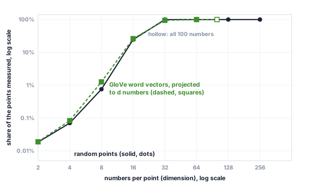
Mia’s ten hand-picked numbers sit between the measured 8 and 16 dimensions, so the tree would measure between a little under one in a hundred and one in four. At five hundred, the tree measures every place, as the scan does, about \(nd\) steps, and on top it keeps a queue of up to \(2n - 1\) regions. On Fashion-MNIST, 60,000 photographs of clothes at 784 numbers each, that made it more than ten times slower than the scan.
In many dimensions, space stops behaving the way your eyes, trained on two and three, expect, and every idea built on that intuition so far stops working. This is the curse of dimensionality [8, p. ix]. Figure 4.14 shows four ways it is odd, on 4,096 points spread evenly in a cube and one question.
Slide the figure to ten, as many numbers as your café had, and then to five hundred.
Volume runs away from the center. The square stands for the cube. Blue is the largest ball that fits inside it, red the smallest ball around it. Blue still touches the middle of every face, yet its share of the cube falls from 79% at two dimensions to 0.25% at ten and \(1.9 \times 10^{-68}\) % at a hundred. Red still touches every corner, yet along an axis it reaches ten times as far as blue at a hundred dimensions, and holds \(10^{100}\) times blue’s volume. Most of a ball’s volume lies in a thin outer shell. The inner ball that holds half of it has radius 0.71 of the whole in two dimensions, 0.93 at ten and 0.993 at a hundred. The drawing is true in two directions only, toward the middle of a face and toward a corner. Every direction between is bent to fit the page, which is why the balls stop looking round.
Distances become similar. That thin shell is why. Points spread evenly at random sit mostly far out, so the distances from one point to all the others come out nearly the same⬢. From the figure’s question, the nearest of the 4,096 points sits at 0.01 of the farthest distance at two dimensions, and at 0.66 at a hundred. For many kinds of random data, the nearest and the farthest point differ less and less, relative to their size, as the dimensions grow [9], [10, Thm. 2.1]. Clustered data need not bunch this way.
The tree ends up measuring everything. A region stays closed only when its bound is larger than the squared radius of the ball around your ten best so far. On the map that radius was small, and one measured distance closed every region whose bound was larger. In many dimensions the tree runs into blue’s tiny share of the cube. At ten dimensions that share holds about ten of 4,096 points spread evenly, and blue’s radius is half the cube’s side. Blue sits at the cube’s center. The same ball around a question anywhere else reaches past the cube’s walls and holds fewer. So every question’s ten nearest lie about half a side away or farther. For the figure’s question they reach 0.62, and the first cut is only 0.18 from the question, so the ball reaches far across it. The tree measures 16 of the 4,096 points at two dimensions, 1,055 at ten, and every one from twenty-four on. Farther up, the distances are nearly equal, so the ball reaches nearly as far as any point and overlaps every region. With 4,096 points the tree gives up sooner than with the 100,000 of Figure 4.13, which is why its share at ten is a little above one in four.
The last panel is the lifeline.
Angles become nearly perpendicular. Pick directions at random and measure the angle between every two. In two dimensions they spread evenly. At a hundred, 92% of the figure’s pairs lie within 10° of a right angle [11, Thm. 2.8, §2.4.2].
Comparing two points costs one step per number, so comparing a five-hundred-number café with a million others costs five hundred million steps. Could each point carry fewer numbers that still keep its distances?
Take a point of length 1 with a hundred numbers. Its shadow (orthogonal projection) on a random direction is how far it reaches along that direction. The length is spread over a hundred directions, so one squared shadow catches about a hundredth of the squared length. Square the shadows, average them, multiply by 100, and you have a guess at the squared length, 1. One shadow guesses wildly. More shadows settle, for the reason the distances bunched. A sum of many small independent pieces stays close to its average, and a squared distance adds one piece per number, as this guess adds one per shadow.
| shadows | five draws | typically off by |
|---|---|---|
| 1 | 0.13, 0.07, 1.45, 0.20, 1.76 | 1.42 |
| 20 | 0.67, 0.51, 0.73, 0.65, 0.82 | 0.30 |
| 80 | 0.98, 1.05, 1.06, 0.92, 0.85 | 0.16 |
Why random directions, and not twenty you pick? Any fixed choice fails for some data. Keep twenty chosen coordinates, and two places that differ only in the other eighty look the same. Random directions can’t be lined up against the data in advance, and in many dimensions they are nearly perpendicular anyway, almost a basis nobody had to fit. Fitting directions to the data is another tool, and the spectral chapter builds it.
Enough shadows keep every length, so every distance between points too. Johnson and Lindenstrauss showed that about \(\log n / \varepsilon^2\) directions, times a constant, keep all distances among \(n\) points within \(1 \pm \varepsilon\), with high probability [12], [13]. The appendix proves it. Giving up a factor of \(1 + \varepsilon\) on every distance to keep fewer numbers is the bargain approximation algorithms make, here applied to search. How many directions it takes depends on how many points there are and on \(\varepsilon\), not on how many numbers each point started with. A million points kept within 10% still need tens of thousands, more than GloVe’s hundred and too many to help the tree. The next section uses random directions directly.
What beat the tree is not the count of numbers. It is how many directions the points really spread in, their real dimension (intrinsic dimension). Clustered data spreads in few, and there a tree can still rule regions out [10, Ch. 2–3]. GloVe’s words spread in many. At their full hundred numbers the tree measured every one, slower than a scan but never wrong, as its box’s Assumes line warned.
No method is known that finds the exact nearest in much less than one measurement per point, even after any reasonable preparation [14, Sec. 1]. The frontier map says why. The searches below are approximate nearest-neighbor search. They give up exactness, and measure how often they are right.
4.7 Places like each other share a code
Locality-sensitive hashing
If cutting the space can’t rule regions out, turn the problem around. Don’t search for the places near Mia’s café when she asks. File every place in advance, so that places alike tend to land in the same drawer, a bucket, and when she asks, look only in hers. Like the k-d tree, this cuts space into compartments. Unlike it, the cuts are random, ignore the places, and are made many times over.
Draw eight cafés as points around the center of a page, and three lines through the center. For each café, write three letters, L or R, for which side of each line it is on. Mia’s café gets three letters too. Which cafés share all three of hers? Is the café most like Mia’s among them? Draw three new lines and do it again.
Ten minutes. You’re done when you can say why one set of lines is not enough, and what a second set adds.
A hash table, from the contracts chapter, files each key under a number computed from the key, so two equal keys always meet in the same place. Near keys don’t, because a good hash is built to scatter. Two cafés that differ only in price, 3.0 against 3.1, are as likely to share a bucket as two cafés that have nothing in common. Equal is the only kind of alike a hash table can see.
So what would a hash have to do to put near things together? And two places can share a bucket without being alike at all. What must you still do with what you find in her bucket?
4.7.1 One random cut, one bit
Pick a direction \(r\), five hundred numbers, each drawn at random⬢ from the normal distribution with mean 0 and variance 1. The cut is the flat sheet through the origin at right angles to \(r\). On a page, it is a line. A place’s bit says which side of a random cut through the origin⬢ it lies on. Multiply the place’s numbers by \(r\)’s, one by one, and add. That is the dot product. Divided by the length of \(r\), it is the place’s shadow on \(r\), so the bit is the sign of a shadow. The bit is 1 when the dot product is zero or more, and 0 when it is negative. On a page this is the hull’s side test again, asked of a line through the origin.
Why would that put near places together? Two places at an angle \(\theta\) from each other, seen from the origin, get different bits only when the cut passes between them. A cut whose direction is drawn at random passes between them with probability \(\theta / \pi\), so their bits agree with probability
\[1 - \frac{\theta}{\pi}.\]
Two cafés pointing almost the same way nearly always agree. Two at right angles agree half the time, like a coin.
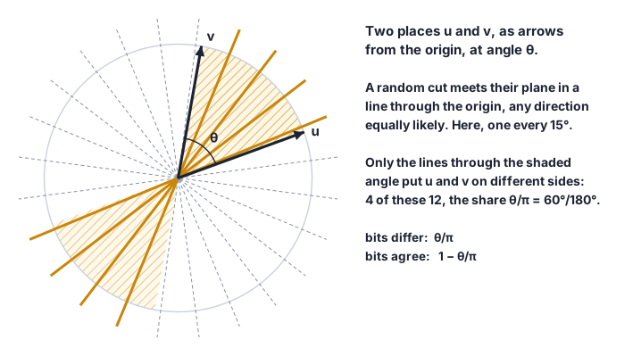
Only the two places and the origin matter, and they lie in one flat plane. The cut meets that plane in a line through the origin (or contains the whole plane, which happens with probability 0). Draw both places as arrows from the origin, at angle \(\theta\).
Each coordinate of \(r\) is drawn from the bell curve, the normal distribution, and that makes every direction equally likely. The direction of \(r\)’s shadow on the plane is just as even. So the cut’s line through the origin points in a uniformly random direction. A line through the origin separates the two arrows exactly when it passes through the angle between them. Its two ends sweep the circle together, so of the half-turn of directions it can take, the share that separates them is \(\theta / \pi\). Otherwise both arrows lie on one side, and their bits agree [15, Sec. 3].
Work out a few bits by hand, on a page, with small whole numbers for the directions (the library draws them at random). Give every café a list of just two numbers, so it can be drawn on a page. Mia’s Lisbon café is \((-7, 1)\) and a café h is \((-7, -1)\). Take the cut with direction \((0, 2)\). Mia’s dot product is \((-7) \cdot 0 + 1 \cdot 2 = 2\), so her bit is 1. h’s is \((-7) \cdot 0 + (-1) \cdot 2 = -2\), so its bit is 0, and this cut runs between them. Add two more cuts, with directions \((3, -1)\) and \((-1, 2)\). Mia gets \(-22\) and \(9\), a 0 and a 1, and h gets \(-20\) and \(5\), a 0 and a 1 as well. In the order \((0, 2)\), \((3, -1)\), \((-1, 2)\), Mia’s three bits read 101 and h’s read 001. Two places close together, and still one cut of three split them.
In the code, a table’s cuts are a list of directions, each coordinate drawn from the bell curve by a seeded generator. The whole module is in lsh.py.
A key of \(K\) bits is shared only by places that agree on every one of its \(K\) cuts, which happens with probability \((1 - \theta/\pi)^K\). A café at 45° from Mia’s is a close one, since most places sit near right angles to hers (the angles panel). With eight cuts, it shares her key one time in ten, since \(0.75^8 = 0.10\). One at right angles shares it one time in 256. A longer key keeps the far places out of her bucket, and keeps many near ones out with them.
4.7.2 Many tables, then check
One table misses a near place now and then, when one of its cuts falls between it and Mia. Tables with their own random cuts miss independently, so a place one table misses is rarely missed by all. Build several. Each of \(L\) tables gets its own \(K\) cuts and files every place under its key there. When Mia asks, every place that shares her key in any table is a candidate. Before anything is reported, the distance from Mia to every candidate is measured exactly, so every distance LSH reports is the true one. Rabin–Karp did the same in the strings chapter. It compared every fingerprint match with the text itself. But equal windows always share a fingerprint, so Rabin–Karp never misses a match. A near place can share no bucket with Mia, and then LSH misses it. With \(K = 8\) and \(L = 64\), the café at 45° becomes a candidate with probability 0.999, and the one at right angles with probability 0.22.
A place at angle \(\theta\) misses one table’s key with probability \(1 - (1 - \theta/\pi)^K\), and it has to miss all \(L\) tables to stay out, so it becomes a candidate with probability
\[1 - \Bigl(1 - \bigl(1 - \tfrac{\theta}{\pi}\bigr)^K\Bigr)^L.\]
Here is the procedure by hand, on eight cafés drawn on a page.
- Mia’s café, \(q = (-7, 1)\)
- a \((-5, 5)\), b \((5, 5)\), c \((-1, 7)\), d \((5, -5)\)
- e \((1, 7)\), f \((-5, -5)\), g \((1, -7)\), h \((-7, -1)\)
All nine lie on one circle around the center, so the café nearer to Mia’s by squared distance is also the one nearer by angle. Two tables, three cuts each. Table 1’s cuts are the three you just worked, so Mia’s key there is 101 and h’s is 001.
| table | cut directions | buckets | Mia’s key |
|---|---|---|---|
| 1 | \((0, 2)\), \((3, -1)\), \((-1, 2)\) | 111 {b}, 101 {a, c, e}, 010 {d, g}, 001 {h}, 000 {f} | 101 |
| 2 | \((-3, -1)\), \((-1, 3)\), \((-3, -2)\) | 111 {a, h}, 101 {f, g}, 010 {b, c, e}, 000 {d} | 111 |
Look in table 1 first. It makes a, c and e the candidates and measures the squared distance from each to Mia’s café, a 20, c 72 and e 100. Alone it would answer a and miss h, because the cut \((0, 2)\) runs between Mia and h. Table 2 is the second chance. It adds h, at 4, and with both tables the answer is h, the true nearest, as the scan over all eight agrees. Four of the eight cafés, b, d, f and g, are never measured at all. On a page, random cuts through the center slice the plane like a pizza, and the places in one slice share a key.
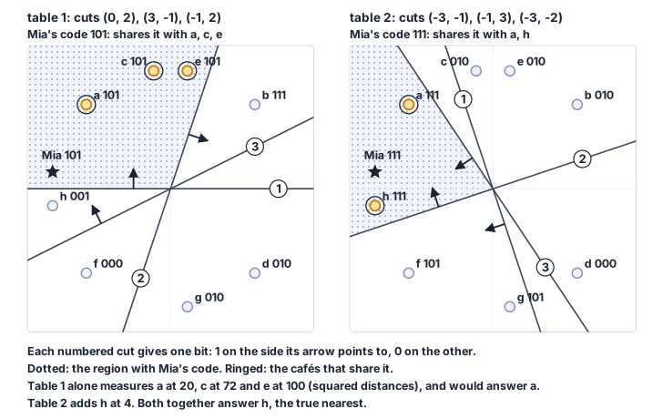
The index files every point in every table, and a query gathers its candidates from all of them and measures each one exactly.
k_nearest_among is the scan’s heap of the \(k\) best, run over the listed points only. Move Mia around below, and before each table finishes her key, say whether it will catch her true nearest café. Then see which tables catch it and which miss it.
This is locality-sensitive hashing, LSH for short [16], [17], and this kind, one bit per random cut, is SimHash [15]. When “near” means straight-line distance rather than angle, the same frame works with a different hash. Cut a random line into equal cells and use the cell a point’s shadow falls in [18]. The appendix shows that grid.
4.7.3 What it costs, measured
LSH wins when the near places are much nearer than the rest, near-duplicates. A place at 5° keeps an 8-bit key with probability \((1 - 5/180)^8 \approx 0.80\), so a few tables find it, while unrelated places almost never collide. Google’s crawler used SimHash this way, on 8 billion web pages. Each page got a 64-bit fingerprint, as in the strings chapter, but one in which near pages differ in few bits. A page whose fingerprint differed from a stored one in at most 3 bits was set aside as a near-duplicate [19]. LSH escaped the count of numbers but not the gap, since its work grows as the near places get less near than the rest [16]. GloVe is the hard case. A word’s true neighbors are not much nearer than everything else, and there LSH loses to the plain scan. The next section’s index reaches the same recall on it more than eight times faster than LSH.
On GloVe, with every candidate re-checked exactly and the first 1,000 questions asked, the library’s SimHash index was measured over a grid of key lengths and table counts. Of all the settings tried, one reaches recall 0.9 or more, eight bits a key and 64 tables. It reaches recall 0.976, measuring 39% of the data, and runs at less than half the scan’s speed on the same 1,000 questions. Measuring two places in five, scattered across memory, cost more than reading all of them in order.
Longer keys or fewer tables answer faster and find less. The formula above shows that trade. With eight bits and 64 tables, a place at 45° almost surely becomes a candidate, but so does one place in five at right angles, and there are far more of those. With sixteen bits, a place at right angles almost never gets in, and a place at 45° gets in only about half the time.
Multi-probe LSH also looks in the buckets next to Mia’s, the ones a near place most likely fell into, and reaches the same recall with fewer tables [20].
Eight bits and 64 tables measured about 460,000 candidates per query. Lengthen the key to 16 bits and the index runs nearly fifty times faster, at recall 0.308. Keep eight bits and drop to 16 tables, and it runs three times faster, at recall 0.655. Computing all 64 keys takes 0.03% of a query. The time goes into measuring candidates.
4.7.4 What a guarantee costs
Once points have many numbers, no known index promises the exact nearest every time much faster than the scan, and one that did would contradict a widely believed conjecture (why). LSH promises a miss chance you can bound, for a nearest within the angle you name, and the promise holds for every set of places, because the only chance in it is the random cuts. Rabin–Karp’s random prime worked the same way in the strings chapter. A text can be written to fool one fixed prime, but not a prime drawn after the text is written. Places can be laid out to fool one fixed set of cuts, but not cuts drawn after the places are given. Every table is another independent try. With 8 bits, a place at 45° shares Mia’s key in one table with probability \(0.75^8 = 0.10\), so each table misses it with probability 0.90, and the misses multiply.
| tables | chance a nearest at 45° is missed |
|---|---|
| 1 | 0.90 |
| 8 | 0.43 |
| 16 | 0.18 |
| 32 | 0.034 |
| 64 | 0.0012, once in 855 questions |
| 128 | 0.0000014, once in 731,000 |
Doubling the tables squares the chance of a miss. So the risk is bounded, and you set the bound. Name an angle and a risk, and the formula says how many tables it takes. A nearest closer than 45° is missed even less often. One farther out is missed more often, by the same formula at its own angle. Each table costs memory and adds candidates to measure. On GloVe, 64 tables bought recall 0.976, at the price of measuring two places in five.
4.8 Ask the locals
Graph index
In her first weeks Mia found most things by asking. The woman at the pharmacy sent her to a bakery by the market. The baker said the café by the river was quieter. The river café’s owner named a third, and that one had plants. Nobody she asked knew the whole city, and each of them knew a few places like their own. Each answer took her a step closer to what she wanted.
Twelve points each know the points they are linked to (Figure 4.18).
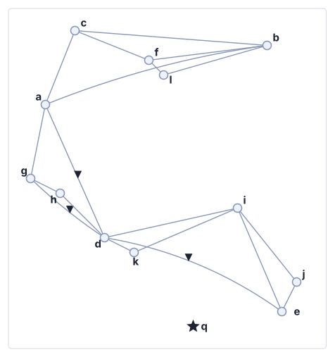
Start at a and walk toward \(q\), always stepping to the linked point nearest \(q\), and stop when no linked point is nearer than where you stand. Where do you stop? Is it the nearest point? Which one link would have let you reach it?
Ten minutes. You’re done when you have the stuck walk, the true nearest, and one link that unsticks it.
To check distances by hand: a \((2, 15)\), b \((17, 19)\), c \((4, 20)\), d \((6, 6)\), e \((18, 1)\), f \((9, 18)\), g \((1, 10)\), h \((3, 9)\), i \((15, 8)\), j \((19, 3)\), k \((8, 5)\), l \((10, 17)\).
LSH’s cuts ignored the places, which is why its promise holds for any set of them. The locals work the other way round. Every link is picked from the places themselves, so the graph follows the data’s shape.
Go back to the map of who is nearest (Figure 4.10), drawn there for the k-d tree’s twelve points, with a cell around every point. Link each point to the points whose cells share a wall with its own. Then a walk that always steps nearer the target always arrives. If you are not standing at the nearest point, some neighbor across a wall is nearer [10, Sec. 6.2]. But in hundreds of dimensions the cell of a random point touches almost every other cell, and a point would need nearly everyone as a neighbor.
Every link costs memory, and every step of the walk measures the distance to each link of the place it stands on. A place linked to nearly everyone makes every step a scan. So each place can keep only a few links, and the walk you just took shows how a few links can fail. A place’s nearest neighbors are the obvious ones to keep, and keeping only them strands the walk in another way. Where places come in clumps, a place’s nearest few sit in its own clump, and a walk that enters a clump may find no link that leads out. Which of a place’s nearest neighbors tell you nothing new?
The first two invariants make the graph flat, a single layer of links. The third adds the layers, and they wait until the flat graph works.
4.8.1 Keep the neighbors that tell you something
Figure 4.19 shows a place a and six candidates for its neighbors, b to g, a smaller set than the twelve points. It may keep at most \(M = 3\). Go through the candidates nearest first, by squared distance from a: b 2, g 13, d 20, c 37, f 45, e 61.
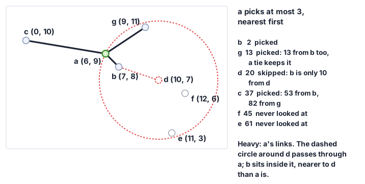
- b is the nearest, so a picks it.
- g is 13 from a and 13 from b. b is not strictly nearer to it, so a tie keeps g.
- d is 20 from a, but only 10 from b. A walk that reaches b is already close to d, so b covers that direction, and d is skipped.
- c is 37 from a, 53 from b and 82 from g. Nothing picked is nearer to it than a is, so a picks it.
Three picked, b, g and c, and f and e are never looked at. Kept this way, a place’s few links point in different directions⬢, and a walk that arrives there can leave toward wherever the target lies. A graph on which such a walk always reaches the nearest is navigable.
In the code, the candidates come in as pairs, squared distance and point number, nearest first. The whole module is in hnsw.py.
4.8.2 Walking toward the target
Now walk it, from a toward \(q = (12, 0)\), always stepping to the linked point nearest \(q\). This is the greedy walk, the walking downhill of the box’s Assumes line. The library linked these twelve points by the rule above. The walk goes a → d → k and stops there. Both of k’s links, d and i, are farther from \(q\) than k is. The nearest point is e, one link beyond i. One more link, d–e or k–e, would have unstuck the walk, and the insertion further down shows how d lost exactly that link.
So keep more than one place in hand. A beam of width 3 keeps the three best places seen so far and expands them nearest first. It measures every neighbor of the place it expands, and keeps a neighbor that beats the worst of the three. It stops when the nearest place not yet expanded is farther than the worst of the three. Here it ends with e, k and j, and finds e.
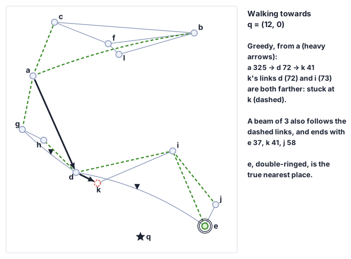
Press q = (12, 0), set the beam to 1, and step. Then set it to 3 and step again, and before each step, say which place it expands next.
This is best-first search again, the k-d tree’s queue with the regions replaced by places. But a region’s bound is never more than the distance to any point inside it, so the k-d search never skips a nearer point. A place’s distance promises nothing about the places beyond it, so the beam can stop before the nearest.
Here dist measures a place’s squared distance to the query, the beam’s width is ef, and lc is the layer, always 0 on a flat graph. found keeps its pairs negated, so its heap has the worst place on top.
The search ends with one more step, finish, which sorts the beam by exact distance and keeps the \(k\) nearest. With ef set to 1 the beam is the greedy walk.
4.8.3 Building it one place at a time
The graph is built by inserting the places one at a time, and each insertion uses the two pieces you already have. A beam finds the new place’s candidates, and the picking rule chooses among them. In the library’s graph a new place picks \(M\) neighbors, and every place’s neighbor list on the bottom layer may hold up to \(2M\). Each picked neighbor links back to the new place. When a list grows past its limit, its owner picks again, by the same rule, from the places it now holds.
Watch the ninth point, i at \((15, 8)\), go into the graph of the first eight, with \(M = 2\), so a list may hold four. The beam finds i’s candidates, nearest first: e 58, d 85, b 125, f 136, h 145, g 200, a 218, c 265. Picking two, i keeps e, and then d, which is 169 from e and only 85 from i.
Now the links back. e had one link, to d, and gets i as its second. d already had four, a, e, g and h, and i makes five, one too many. So d picks again from its five, nearest to d first: h 18, g 41, i 85, a 97, e 169.
- h is the nearest, so d keeps it.
- g is 41 from d but only 5 from h, so d skips it.
- i is 85 from d and 145 from h, so d keeps it.
- a is 97 from d but only 37 from h, so d skips it.
- e is 169 from d but only 58 from i, so d skips it.
d ends with h and i. A re-pick can shrink a list, never grow it past the limit.
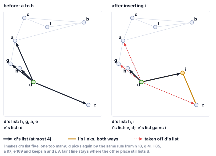
Look at e and d afterwards. e still links to d, and d no longer links to e. Links are made in both directions, as the box says, and a re-pick can drop one of them. That is why Figure 4.18 draws e’s link to d with one arrowhead.
Press Next step to watch the twelve places go in, from a to l, with \(M = 2\) and the levels from seed 2. Before each step, say which places the new one keeps, and whether any list overflows. The ninth insertion is the one above, number for number.
In the code, the loop runs over every layer the new place reaches, from the top one down. On a flat graph that is only layer 0, and entry_points is where the search starts, the first place inserted.
The lines left out give the new place an empty list on each of its layers, make the very first place the entry and stop there, and otherwise walk greedily down from the top layer to the first one the new place is on.
4.8.4 Highways
So far every walk starts at the first place inserted, wherever that is. In a city, nobody walks to the other side of town through the side streets. You take a highway most of the way, and the side streets only at the end.
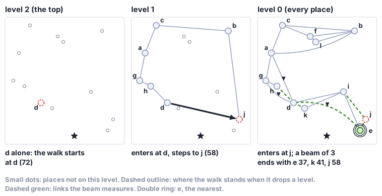
The library’s graph builds its own highways. Each place draws a level at random when it is inserted, and few draw a high one. Each layer up keeps a random few⬢ of the one below, about one place in \(M\). A place is linked on its own level and on every level below it. A search starts at the single entry place on the top layer, walks greedily on each layer until it is stuck, drops to the layer below where it stands, and runs the beam only on the bottom layer, among everyone. This is the hierarchical navigable small world graph, HNSW [21]. The same layering over sorted keys is the skip list, in the search chapter’s frontier map.
Build the twelve points this way, with \(M = 2\) and the random levels from seed 2. d alone reaches level 2, and is the entry. Level 1 holds d, a, b, c, g, h and j, linked as Figure 4.24 draws them. Level 0 holds everyone, with the same links as the flat graph from the start of this section. Walk to \(q = (12, 0)\) again. On level 2, d has no links, so the walk stays at d, 72. On level 1, d’s links are h at 162 and j at 58, so it steps to j, and j’s links, d and b at 386, are both farther, so it drops at j. On the bottom layer, from j, a beam of 3 ends with e 37, k 41 and j 58, and finds e. The highway moved the start from a to j, close enough that even the greedy walk would now reach e, since j’s links include e.
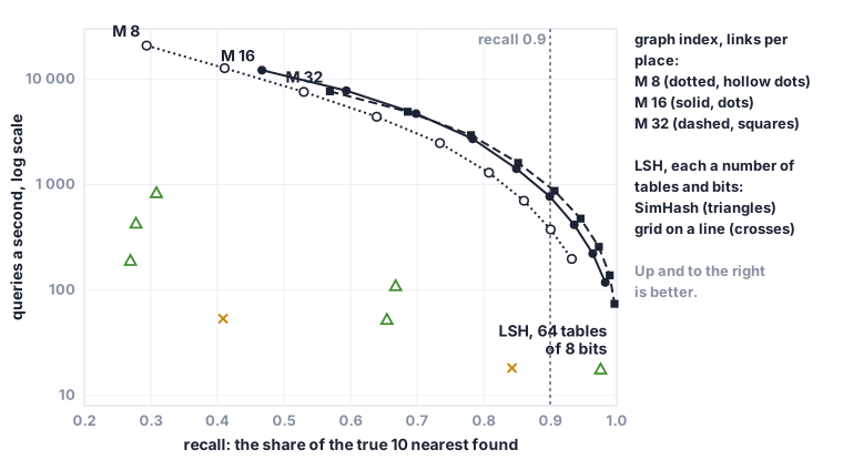
On GloVe, with \(M = 16\) and a beam of 200 while building, all 1,183,514 words and all 10,000 questions, the layered graph and the flat one reach the same recall at the same speed, within a few percent at every beam width. Building the same layered graph a second time moves its speed about as much. At this size and in a hundred dimensions, the highways buy nothing that can be measured.
Munyampirwa and his co-authors found the same on their data, and traced it to hubs. In many dimensions a few places turn up in almost everyone’s lists, and they serve as highways on their own [22]. The library ships the layers anyway, as the standard design does, since the flat graph saves so little.
4.8.5 What it costs
The beam’s width, ef, is the setting Mia’s service tunes. The default graph has \(M = 16\) and was built with a beam of 200. Table 4.6 shows what each width buys on GloVe.
| ef | 10 | 40 | 160 | 640 | 1,280 | 2,560 |
|---|---|---|---|---|---|---|
| recall@10 | 0.467 | 0.699 | 0.849 | 0.936 | 0.964 | 0.983 |
| questions a second | 12,168 | 4,712 | 1,413 | 416 | 222 | 118 |
Each fourfold widening of the beam, from 10 up to 640, leaves about a third of the speed, and each doubling after that about half, and each buys less recall. More links buy speed with memory.
At recall 0.95, read between two measured beam widths, \(M = 32\) answers about 430 questions a second and \(M = 16\) about 300. \(M = 32\) needs 1.5 times the memory of \(M = 16\) and 1.6 times its build time. With \(M = 8\) no beam up to 2,560 reaches 0.95. Its best is 0.932. The order the words go in barely matters. In the order of the file, the recall stays within 0.005 of a shuffled order’s at every width.
At LSH’s recall of 0.976, read between two measured beam widths, the graph answers more than eight times as many questions a second as LSH.
Over all 10,000 questions LSH reaches recall 0.9763. The two measured beam widths around it answer 221.7 questions a second at recall 0.9640 and 117.9 questions a second at recall 0.9828. Recall 0.9763 lies 65% of the way from 0.9640 to 0.9828, so on a log scale of speed the graph reads as \(221.7 \times (117.9/221.7)^{0.654} \approx 147\) questions a second. LSH answers 17 questions a second.
All of that keeps every vector in memory. On a phone asks what happens when they don’t fit.
Mia’s phone can’t hold five hundred numbers for every place on a continent. The library keeps every number in 8 bytes, so GloVe’s hundred numbers take 800 bytes a word, 947 MB for all of them. So keep one bit per number instead.
First rotate every vector at random around the data’s center. This is the shadows’ idea again, a random change of directions, so that no coordinate is special. Then keep only the sign of each rotated number. That sign is SimHash’s bit again, from a cut through the data’s center, with the directions now at right angles to one another. Rounding numbers to a few bits like this is quantization. Keep two numbers per vector besides, which correct the estimate. RaBitQ [23] estimates every distance from those bits without bias, right on average. The bits and the two numbers make a vector’s short code, 32 bytes instead of 800. The 100 bits are stored in two 64-bit words, 16 bytes, and the two correcting numbers take 8 bytes each. The walk ranks places by these estimates, and at the end it measures exactly the ef places it holds. As in LSH, a cheap filter comes first and an exact check after. The query is rounded to a few bits too, which is where the speed comes from. How the estimate is computed from the bits stays a black box here. The spectral chapter returns to short codes for vectors, built from clusters of the data.
When everything fits in memory, the estimates lose recall, and the beam has to be wider to make up for it, so the full vectors win. They are up to about twice as fast at equal recall. To see the phone’s side, the library ran the same graph and codes with the process capped at 450 MB after building. The 947 MB of vectors alone are twice the cap, so the vectors were read back from the disk as the walk touched them. Then the codes were about three and a half times faster at equal recall.
The paper pairs its codes with an index that groups the vectors into clusters, and proves its guarantee for the exact re-check there. That guarantee doesn’t carry over to a graph.
4.8.6 What it cannot promise
The box promises only what it can check. It returns up to \(k\) places, nearest first, each measured exactly. Nothing in the design says the walk reaches the true nearest, and for this kind of graph no such guarantee is known. On inputs built for the purpose, several popular graph indexes were measured to need query time that grows in step with the size of the data before they reach reasonable accuracy, and HNSW, the design built in this chapter, is among them [24]. The search chapter’s frontier map points to the same result. So recall is measured instead, on a named dataset, and it holds for that data and no other. When the walk stops at a place that is not the nearest, the answer is wrong and looks exactly like a right one.
The library states each design in the proof assistant Lean, one file per structure, KDTree/Spec.lean and GraphIndex/Spec.lean for the two halves of this chapter.
For the k-d tree, the build is proved to keep both of its cut invariants, and the search to return exactly the scan’s \(k\) nearest, on any points. Which point wins a tie, and leaves that hold more than one point, are tested, not proved, because the Lean’s leaf holds a point, not its number.
For the graph, every insertion is proved to keep the limit on every list and the layers nested, whatever candidates the search hands it, as long as they are places already on that layer, each named once. So that proof does not depend on the walk being any good. Every picking is proved to follow the rule. And the search’s last step is proved to return the beam’s \(k\) nearest, each measured exactly. The walk that fills the beam is modeled too, step for step, and proved to hand that step stored places, each once. Whether it finds the true nearest is not a theorem but a measurement, recall.
The first half’s answers are proved to be the scan’s. The second half’s are measured against it. And no proof says whether five hundred numbers from an AI were the right way to say what Mia’s café was like. That question stays with whoever asks.
4.9 ✎ When the ground shifts practice
A service holds ten million descriptions, 768 numbers each, and must return the ten most alike in a few milliseconds. A colleague proposes a k-d tree, “because it measured about four points out of a million, on a map of points spread evenly”. Say whether it fits, and what you would measure first, on which data, before anyone writes code.
This check needs the fold On a phone, in the graph index’s section. Read it first. The same service moves to phones. The vectors no longer fit in memory, and most of them stay on the disk. Which of the chapter’s measurements stop describing it, and which design comes out ahead instead? Say what the short codes of On a phone cost when the vectors do fit, and why that cost changes sign when they don’t.
The places start to move. Delivery drivers each report where they are every few seconds, and a restaurant asks for the nearest five. For each structure in the chapter, say which assumption of its box this breaks, and whether the answers become slow or wrong. Then say which structure you would rebuild from scratch every few seconds, and what that costs.
4.10 ◆ What these are actually made of big picture
This chapter built a scan, two trees, a fence, a hash and a graph. Open them up, and they are made of a handful of small ideas, several of which turn up twice inside the chapter, and some of which you met earlier in the book doing other jobs.
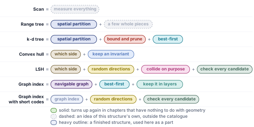
Scan = measure everything. No preparation, nothing to keep true, and every question measures every place. Every structure after it is a way not to, and every one of them is checked against it.
Range tree = spatial partition + a few whole pieces. Spatial partition: sort once and split the line in halves, so any range is a few whole subtrees and two paths. A few whole pieces: each subtree between the two paths is reported without testing any of its keys.
k-d tree = spatial partition + bound and prune + best-first. The partition cuts the map itself, by turns. Bound and prune: a region’s bound is never more than any of its points’ distances, so a region whose bound is already too far stays closed. Best-first: open the region with the smallest bound next, so a good answer comes early and the bounds stop the search soon after.
Convex hull = which side + keep an invariant. Which side: the sign of one number says whether three points turn left. Keep an invariant, here a loop invariant: what the chain keeps turns left at every point, and each new point restores that before the next one comes.
LSH = which side + random directions + collide on purpose + check every candidate. The hull’s question again, asked of a cut through the origin. Random directions: the cuts know nothing about the places, so no set of places can fool them every time. Collide on purpose: where an ordinary hash scatters, this one files near places together. Check every candidate: a shared bucket only makes a place a candidate, and only an exact distance decides, as Rabin–Karp’s match was checked against the text in the strings chapter.
Graph index = navigable graph + best-first + keep it in layers. Navigable graph: a few links per place, pointing in different directions, so a walk that always steps nearer gets somewhere. Best-first again: the beam is the k-d tree’s queue, with places where the regions were. Keep it in layers: a random few on each layer up, so a search starts on a small layer and ends on the full one, as the LSM-tree in the search chapter put a small table in front of its large levels. On a phone, the graph index with short codes adds random directions, the rotation before the signs are kept, and checks every candidate the codes rank, exactly, at the end.
4.10.1 Choosing one, under pressure
Every structure here makes a promise. Break what a right answer needs and the answers are wrong. Break what makes it a good choice, and the answers are still right, but you are paying for the wrong thing. Each row is a short contract, in the contracts chapter’s sense. The last column is its failure mode, what you see when either one breaks. In most rows you see no error at all, just an answer that looks exactly like a right one.
| structure | a right answer needs | it is a good choice when | if it breaks |
|---|---|---|---|
| Scan | nothing | the places are few, change all the time, or are asked about once, or an index would still measure a large share of them | it is never wrong, only slow |
| Range tree | the places don’t change after the build | “everything in this strip”, or in this rectangle with two coordinates, is asked often | a place added after the build is never reported |
| k-d tree | the places don’t change after the build | the nearest place on a map, asked millions of times, where the points really spread in only a few directions | a place added after the build is never found. With many real dimensions it stays right but slows down, and on points spread evenly it measures nearly every point at 32 numbers and every point from 64 |
| LSH | cuts drawn at random, knowing nothing about the places | you need a risk bounded in advance: a nearest within the angle you name is missed at most as often as you set | a farther place, silently, when the true nearest shares a bucket in no table |
| Graph index | walking downhill through the neighbors leads to the nearest | millions of places, hundreds of numbers each, at a recall you choose and measure | a farther place, silently, for instance when a condition like open now removes places the walk needed to pass through |
4.10.2 What each one costs
This finishes the ledger of What has been bought so far. Each point has \(d\) numbers, there are \(n\) of them, and \(k\) are reported. LSH keeps \(L\) tables with keys of \(K\) bits, and the graph keeps \(M\) links per point.
| structure | prepare | one question | memory | measured |
|---|---|---|---|---|
| Scan | nothing | \(\Theta(nd)\) | the points, \(\Theta(nd)\) | about 39 questions a second, on GloVe, 1,183,514 words of 100 numbers, the first 1,000 questions |
| Range tree, two coordinates | \(O(n \log n)\) | \(O(\log^2 n + k)\) | \(O(n \log n)\) | not measured |
| k-d tree, one point per leaf | \(O(dn \log n)\), a sort per axis first | \(O(n)\) regions in the worst case, all \(2n - 1\) | \(\Theta(n)\) nodes, plus the points | 3.93 points measured per question, about 830,000 questions a second, on 1,000,000 points spread evenly over a square |
| LSH, 8 bits, 64 tables | \(\Theta(nLKd)\), a key per table per point | \(\Theta(LKd)\) for the keys, plus \(d\) per candidate | \(\Theta(nL)\) entries, plus the points | 39% of the data measured, recall 0.976, less than half the scan’s speed, on GloVe, the first 1,000 questions |
| Graph index, \(M = 16\) | no proven bound, each insertion a beam search | no proven bound | \(\Theta(nM)\) links, plus the points | about 300 questions a second at recall 0.95, on GloVe, all 10,000 questions |
| Graph index with short codes | a code per point | the graph’s walk on the codes, then an exact check | 32 bytes a point, beside the graph | about three and a half times the full vectors’ speed at equal recall, when the vectors must be read from disk, on GloVe, 200 questions at each beam width, with the process held to 450 MB |
Only the top half of the table is exact. The scan, the range tree and the k-d tree return the true answer every time, and their costs differ. LSH and the graph index return an answer measured exactly, and how often it is the true one is one more number, recall, that holds only for the data it was measured on.
The k-d tree’s row is a fact about a map. On the first 100,000 GloVe words, at their full hundred numbers, the same tree measured every word. On Fashion-MNIST, 60,000 small photographs of clothes at 784 numbers each, over its first 1,000 questions, it ran more than ten times slower than the scan. A row of this table carries its data with it.
Memory decides the last row. With every vector in memory the full vectors walk faster. With the vectors on the disk, the codes do.
Fewer distances is not less time. LSH measured 39% of GloVe and still ran slower than the scan timed on the same questions, at less than half the scan’s speed. Count distances to compare designs. Time them before you choose.
4.10.3 Where they run
Each of these runs inside programs in daily use.
| structure | where it runs |
|---|---|
| k-d tree | the nearest-neighbor routines of scientific libraries, such as SciPy’s KDTree |
| R-tree, a B-tree for rectangles | the spatial indexes of databases, such as PostGIS |
| Convex hull | geometry libraries, such as SciPy’s ConvexHull, which calls the Qhull library |
| Graph index | vector search in databases and search engines, such as pgvector’s HNSW index and the vector search of Lucene |
| Short codes with an exact check | vector search libraries, such as Faiss, which offers RaBitQ’s codes |
The range tree is missing from the table. Databases answer strips and rectangles with B-trees and R-trees, which keep their nodes in blocks the size of a disk page, as the B-tree in the search chapter did, and which can change after the build.
4.10.4 The same ideas, over and over
| primitive | where else it turns up |
|---|---|
| spatial partition | quadtrees behind map tiles, octrees in 3D graphics, the grids of a physics simulation |
| bound and prune | alpha–beta pruning in chess programs, the solvers of integer programs |
| best-first | Dijkstra’s shortest paths, A* in games, the graph index’s beam |
| which side | the SimHash bit, a linear classifier’s decision, the exact tests inside mesh generators |
| random directions | the sketches of the streaming chapter, randomized methods for large matrices, RaBitQ’s rotation |
| collide on purpose | catching spam sent in many slightly different copies, MUVERA’s buckets in the frontier map |
| check every candidate | Rabin–Karp’s match in the strings chapter and the exact recomputation behind orient2d. The Bloom filter in the search chapter made the opposite choice |
| navigable graph | small-world networks, routing between machines on a network |
When a problem arrives that no structure here fits, ask which of these ideas it needs. What can be cut into regions? What bound can rule a region out? Which question is answered by a sign? And what can you check exactly, once something cheaper has narrowed the field?
4.11 ◆ Where that leaves the pharmacy big picture
Months on, a neighbor knocks late in the evening. Her daughter has a fever. Mia types pharmacy, open now, and five pharmacies appear before her thumb leaves the screen. She knows three of them by name now, and she knows which one has the short queue. The city has stopped being foreign. Perec’s doubt is still there, but she has marked the space, again and again, until it holds her.
The phone answered her two questions in two different ways. On the first night it answered exactly. Nearest meant nearest, and the map made that cheap, because one measurement told the search about a whole region. In month two it answered well enough, nine places in ten like the café in Lisbon, at a speed the service could afford. In five hundred dimensions one measurement rules out almost nothing, so the conclusions the map gave away free had to be bought back, with tables and candidates in LSH and with links and a wider beam in the graph. What they bought back is measured as recall.
And “open now” was a filter all along. On the map a filter never makes the answer wrong. A k-d search can measure a closed pharmacy and pass over it, and every bound still holds, so the answer is still the nearest open one. On the graph, drop the closed places from the walk, and the paths that ran through them are gone. Walk through them anyway, and the beam fills with places it may not report. That is where the walk still breaks today, and where the frontier map below picks it up.
Most of what this chapter named is what the rest of the world calls it too: range query, nearest-neighbor query, range tree, split node, k-d tree, best-first search, Voronoi diagram, convex hull, orientation, embedding, recall, locality-sensitive hashing, SimHash, candidate, HNSW, beam, priority queue, greedy walk, curse of dimensionality, quantization. A few words were this chapter’s own. The shadows are orthogonal projections onto random directions, and together, scaled, they make a random projection. A place like this one is approximate nearest-neighbor search. The real dimension is the intrinsic dimension. The locals are a graph index, and its highways are the layers of HNSW. The picking rule is what HNSW’s paper calls its neighbor-selection heuristic. They were scaffolding, and the ideas underneath keep their standard names.
For a quotation, a citation, or a check that a model copied its training text, a passage that means the same is not evidence. Only an exact match is, and that is the strings chapter’s job.
In two dimensions you can afford exact. In five hundred you choose how wrong you are willing to be, and measure it.
4.12 ✎ Take a turn with the places practice
Projects come first. In each one you build something, measure something, or explain something to another person. They have no single right answer, so nobody can mark them for you. After them comes a bank of numbered exercises, each with one right answer you can check. Do some of each. The exercises show what you know, and the projects show what you can do. Where a project needs code, let an AI write it. The times given assume it does. Three things stay yours even when the AI helps. You say what the code must do, build the check that shows it does, and judge what comes back. In this chapter that check almost always has the same shape. Compare with the scan, and say what data you compared on.
Project 1 · the k-d tree · hard · ~2 hours
Build Mia’s “near me”. Take the pharmacies, or the cafés, of a city you know from a public map extract, or scatter synthetic points over a square and say that you did. Have an AI build a service that answers “the nearest one to here” with a k-d tree. Before you ask, write down these checks.
- on a thousand random questions, the answer is the scan’s answer, and a tie goes to the lower number;
- a map with no points answers nothing;
- a question asked exactly at a point answers that point, or the lower-numbered of two points in the same spot.
Run the checks before you believe a single answer. Then count the points measured per question, and put that number beside the scan’s \(n\). Say what points you counted on.
Project 2 · the range tree · ~1 hour
Pay for the second coordinate. Have an AI build the two-coordinate range tree from Two coordinates at once. Specify the check first. For every rectangle you try, the tree returns exactly the points a plain filter over all of them returns, each once. Then predict how many entries the tree stores, counting every point once in every second tree it belongs to, for 1,000, 10,000 and 100,000 random points. Count them, put each count beside \(n \log_2 n\), and say in one sentence what the second coordinate cost and what it bought.
Project 3 · the convex hull · ~45 min
Your rule, as a test. Turn the rule you wrote in the hull’s Try first into a slow check. A pair of points is an edge of the fence when every other point lies on one side of the line through them. Have an AI write Andrew’s chain. Then break it on purpose, twice. First, keep a point when the turn is a left turn or straight (>= 0 instead of > 0). Second, compute the turn in plain floating point, on points a rounding step apart near a line, as in When the sign lies. Say which of your tests catches which broken version, and whether either escapes all of them.
Project 4 · the curse · ~1.5 hours
Measure the curse on your own data. Pick a dataset of lists of numbers you care about: photos, songs, sensor readings, word vectors. Measure the share of points a k-d search for the ten nearest measures, as you keep more and more of the numbers, the way Figure 4.13 does. Then take points spread over a plane, two numbers each, and turn them into lists of 100 numbers by one random rotation, so they still lie on a flat sheet. Before running either, predict both curves. Hand in the two curves, your predictions, and one paragraph on the difference between how many numbers a point has and how many directions the points really spread in.
Project 5 · LSH · ~1.5 hours
Tune the two settings. On the first 100,000 GloVe words, measure recall@10 and candidates per question for keys of 4, 8 and 12 bits and for 4, 16 and 64 tables, nine settings in all. The true ten nearest come from the scan over those 100,000 words, which you run first. Before measuring the nine settings, predict, from \(1 - \theta/\pi\) and the formula in Many tables, then check, which settings will reach recall 0.9. Hand in the grid of measurements beside your predictions, and say which setting you would ship, and why.
Project 6 · the graph index · ~1 hour
Do highways pay? Build the graph index flat and with layers on 10,000 points, once with 2 numbers each and once with 100, and measure both at the same recall on your own machine. Say in one sentence whether your measurements agree with Highways, and if not, what differs between your data and GloVe.
Project 7 · filters · ~1 hour
“Open now”. Build a graph index over your places, then close half of them at random. Walk the same graph without ever stepping on a closed place, and measure recall@10 at beam widths 10, 40 and 160, against the scan over the open places only. Then walk through closed places but never report them, and measure again. Hand in both tables and one paragraph on why the first walk breaks.
Project 8 · design · hard · ~3 hours
Design an index for “places like this one”, with an AI. Mia’s service answers “places like this one” over places that are each a list of numbers, and it has a memory budget. The scan’s ten nearest are the reference. Find a design that computes at most half the scan’s distances per question, finds on average at least nine of the true ten nearest (recall@10 of at least 0.9), and stays under the memory cap. It has to do all three on every set of places you test it on. The AI writes the code. You specify, check and judge.
The companion library holds a bench for exactly this problem. Its places are 10,000 points of 100 numbers each, drawn from a seed. One family is clustered, and one is built to be hard, with clusters of very different sizes, near-copies of points, and questions that fall between clusters. Each set comes with 100 questions. The bench charges one for every distance and every inner product a candidate computes, whatever it computes them for, and its cap counts the index alone, at most as many numbers as the stored points themselves hold.
- Write the problem first. Write the top half of a box: goal, promise (what every answer must be, and recall measured against the scan’s ten nearest), cost (distances and inner products per question, memory), assumptions. Leave the idea and the invariants empty. They are what the search will find.
- Check the promise where a machine holds it. Read
Contractin the library’slean/AlgoDesign/Geometry/Workbench/Spec.lean, what every answer owes and how recall is counted. Check that each line says what your promise says, and change the contract where it does not. - Hand the top half to an AI, with the bench,
python/algodesign/geometry/workbench.py. A candidate sees the points and each question only through the bench’s countedPointsandQuery. Ask for the code in one language and for its box. The AI may tune onPRACTICE_SEEDS. Keep some seeds to yourself. - Judge what comes back. Run
judgeon your own seeds and read itsreport: recall on the worst seed, distances per question against the scan’s, memory against the cap. Judge the chapter’s own structures beside it,scan_candidate,kdtree_candidate,lsh_candidateandhnsw_candidate. - Repair, and say why. Each time something is wrong, decide whether it is the code, the box, or the design, and write one line saying which and why.
Hand in the final box, whole, the lines from step 5, and the measurements. ★ Prove in Lean that your design meets Workbench.Contract.
Another brief or another AI gives another run. This is one.
Round 1. Checked against Contract, the promise matched it field for field, and nothing changed. The check did show that an answer of no places at all keeps the contract, and only recall stops it. The box asked for at most half the scan’s distances and inner products per question. The AI picked fifty landmark places and gave every place fifty-one numbers worked out from its distances to them, 510,153 numbers in all, about half the cap. A question measures the landmarks, works out from those numbers a lower bound on its distance to every place, and measures places in order of their bounds until no bound is below its tenth nearest. On the hidden seeds it found all ten every time, at 83 or 84 distances a question on clustered places and 610 on the worst skewed set, and every check passed. Its own box said what the count leaves out. Every question works out a bound for all 10,000 places, from numbers the bench does not count. It kept the promise and missed the goal, which was to find similar places without measuring them all. Fix the box: the cost now counts every place a question touches, measured or only read, and what the bench cannot count is checked by reading the code.
Round 2. The AI returned a graph. Each place links to the sixteen nearest it finds, every link both ways, and a question measures 100 starting places spread over the clusters, then walks from the nearest, reading links only of places it has already measured. So every place it touches costs a distance the bench counts, and the code shows it. On the hidden seeds it passed, with recall@10 0.931 on its worst set, 1,630 distances a question on its costliest set, and 259,507 numbers in all. Nothing to repair. Beside it, on the same sets, the chapter’s graph index with layers touched 398 places on its worst set, about a quarter as many, with recall 0.913, closer to the bar. LSH passed at 4,825 distances and inner products a question, 48.3% of the scan against the bar’s half, with recall 0.958, and the k-d tree computed 10,094, more than the scan’s 10,000. Both graphs lost recall on the seeds kept back, the AI’s from 0.983 on the practice seeds it was tuned on and the chapter’s from 0.954. A bar checked only on the seeds you tuned for promises more than it keeps.
Along the way the AI noted that the memory check catches coordinates copied as they are, not the same places written in other directions. Enough landmarks would hold nearly all of every place, still under the cap. Round 2’s box already charges for that, since a question that reads those numbers touches the place. A check catches only what it looks for, and the check you build is part of the design too.3
Here is the range query from Where the two ends part, written the way many people first write it. Two tests have changed. The walk to the split node goes left when hi is at most the node’s key, and hi’s walk reports a left child only when the node’s key is strictly smaller than hi.
while isinstance(v, Node) and (hi <= v.split or v.split < lo):
    v = v.left if hi <= v.split else v.right
...
w = v.right                    # hi's walk, right of the split node
while isinstance(w, Node):
    if w.split < hi:
        found.append(w.left)
        w = w.right
    else:
        w = w.left
It reads naturally. A node’s key is the largest key on its left, so a range that ends at that key seems to lie wholly on the left. Every test with distinct keys passes, which is why this version gets published.
- Before running anything, say which keys this version can leave out of an answer, and why no test with distinct keys can catch it. Keys in the leaves has the reason.
- Write the smallest input that shows it, the keys and one range. Smallest means fewest keys.
- Now take the keys 3, 3, 3, 3, 3, 1, 5. Say what this version returns for the range from 3 to 3, and for the range from 0 to 3, and what each should return. Then say why the ranges from 3 to 5 and from 2 to 4 come out right.
Only after you have your own answer, hand the lines to an AI and ask what is wrong with them. Does its answer find the problem? Whether <= is wrong here depends on where the build puts copies of a node’s key, a rule that lives in another function, which the AI was not shown.
4.13 ✎ A bank you can mark yourself practice
Here are thirty-nine exercises. Each shows roughly how long it takes, and everything you need for them is in the chapter so far. The answers are on a page of their own.
If you only do four, do Exercises 2, 5, 10 and 12.
They are grouped by kind of task, not by structure. To practice one structure, here are the exercises for each section:
- Everything between two streets: 1, 2, 16, 22, 39
- The nearest one, now: 3, 4, 5, 17, 25, 26, 27, 37, 38
- The part of town she knows: 6, 7, 28
- A place like this one: 8, 29
- Places like each other share a code: 9, 10, 11, 18, 20, 23, 30, 31, 34, 36
- Ask the locals: 12, 13, 14, 15, 19, 21, 24, 32, 35
- What these are actually made of: 33
4.13.1 Run it and report the state
Exercise 1 · gentle · ~10 min
Build the range tree over the keys 84, 71, 69, 42, 20, 46, 86, 30, 54, 36, 75, 40. Sort the keys and hang them in the leaves. Every inner node splits the keys below it in half, the left half taking the extra key when the count is odd, and holds the largest key of its left half. Give the key of every inner node, level by level from the root, and the tree’s depth.
Exercise 2 · middling · ~15 min
In the tree of Exercise 1, query the range [65, 86]. At a node, go left when 86 is smaller than its key and right when its key is smaller than 65. The first node where neither holds is the split node. Which node is it, and which nodes does the walk pass on the way? Then follow 65 down the left side and 86 down the right side: which nodes does each path visit, which whole subtrees does each report, and which keys come out?
Exercise 3 · gentle · ~15 min
Build the k-d tree over the points a (8, 10), b (19, 8), c (4, 15), d (15, 5), e (7, 17), f (3, 1), g (13, 7), h (18, 9), i (20, 16), j (17, 6). Cut on x at the root, then on y, taking turns. At each node the left side takes the first half of its points along the axis (the extra point when the count is odd), and the cut is the coordinate of the last of them. A leaf holds one point. Draw the tree: the cut at every node, and the point in every leaf. How deep is it?
Exercise 4 · middling · ~15 min
In the k-d tree of Exercise 3, find every point with 12 ≤ x ≤ 19 and 3 ≤ y ≤ 12. Keep the region each node covers, bounded by the cuts above it and running on without end where no cut bounds it (not the smallest box around its points): report a region whole when it lies inside the rectangle, skip a side the rectangle does not reach, and open the rest. Which regions are reported whole, which are skipped, which leaves do you check one point at a time, and which points come out?
Exercise 5 · hard · ~25 min
In the k-d tree of Exercise 3, find the point nearest to (9, 11) by best-first search, in squared distances.
- Every waiting region carries a bound: the sum of the squared distances from the query to the region along each axis.
- Always open the waiting region with the smallest bound. Opening a node queues its far side first, then its near side, which keeps the parent’s bound, and equal bounds come out in the order they went in.
- Stop when the smallest bound waiting is larger than the best distance found.
In what order are the regions opened, which points are measured, which regions are skipped, and why?
Exercise 6 · middling · ~15 min
Run Andrew’s monotone chain on the points a (9, 7), b (0, 10), c (3, 4), d (12, 9), e (7, 11), f (4, 5), g (5, 2), h (1, 8). Sort them by x, build the lower chain left to right and the upper chain right to left, and drop the middle of the last two kept points whenever the new point does not make a strict left turn. Which points are dropped, and when? What is the hull, counterclockwise from the leftmost point?
Then: The turn test is written >= 0 instead of > 0. Which point is kept now that the promise says must be left out, and why?
Exercise 7 · gentle · ~5 min
Walking from a to b, is c on the left, on the right, or on the line? Give the sign of the orientation test, once for a (1, 9), b (0, 4), c (3, 0), and once for a (7, 1), b (6, 2), c (0, 8).
Exercise 8 · middling · ~15 min
A box runs from -2 to 2 along every axis. In each of its corners sits a ball of radius 1, centered at the point whose every coordinate is 1 or -1, so it touches the box’s walls at that corner and the balls in the neighboring corners. A ball at the center of the box is made as large as it can be without overlapping any corner ball. What is its radius when every point has 2 numbers, 10 numbers, and 100? From how many numbers on does the center ball reach outside the box, though every corner ball stays inside it?
Exercise 9 · gentle · ~10 min
A table’s cuts are lines through the origin, given by the directions (2, 2), (-1, -3), (1, -1). A point’s bit for a cut is 1 when the dot product of the point with the direction is zero or more, and 0 when it is negative. Its key is its three bits in the order of the cuts. Hash the points a (-4, -3), b (3, 4), c (0, -5), d (4, -3), e (3, -4), f (-3, 4), g (0, 5), h (-5, 0). What is each point’s key, and which points share a bucket?
Exercise 10 · middling · ~15 min
Add a second table to the points of Exercise 9, with the cuts (3, 1), (2, -1), (3, 3). The query is (-3, -4). What is its key in each table, which points share a bucket with it in some table, and which point is the answer after measuring each of them exactly? What would the answer have been with the first table alone?
Exercise 11 · middling · ~25 min
An LSH index uses keys of K = 4 cuts and L = 8 tables. With what probability does a place at 60° from the query share the query’s key in one given table, and with what probability does it become a candidate? Answer the same for a place at right angles to the query.
Then: Choose K and L so that a place at 45° becomes a candidate with probability at least 0.99, and one at 90° with probability at most 0.05, with as few tables as you can. Try key lengths from 4 up, and for each find the fewest tables that let the 45° place in. Keep four decimal places.
Exercise 12 · middling · ~10 min
The place a (9, 8) picks at most 3 neighbors from the candidates b (6, 0), c (0, 12), d (12, 9), e (11, 2). Take them nearest first, in squared distances, and skip a candidate when a neighbor already picked is strictly nearer to it than a is. Which are picked, in order, and which is skipped, because of which neighbor?
Exercise 13 · middling · ~15 min
A flat graph index holds the places a (14, 17), b (4, 19), c (5, 9), d (13, 10), e (1, 11), f (8, 1), g (15, 8), h (16, 16), i (9, 7), j (11, 6), with the links a: b, d, h; b: a, c, e; c: e, i; d: g, i, h, j; e: c, b; f: c, g; g: d, f; h: a, d; i: c, d, j; j: i, d. Walk greedily from a toward the query (12, 0): at each place, measure every neighbor and step to the nearest one if it is nearer than where you stand. Stop when none is. Which places does the walk visit, with their squared distances, and where does it stop? Is that the nearest place?
Then: Walk again from a, but keep the 3 nearest places seen so far: each time, take the nearest kept place you have not yet expanded, measure its neighbors you have not measured, and keep the 3 nearest of all you have seen. Stop when the nearest place not yet expanded is farther than the worst of the 3 kept. Which kept place is nearest to the query?
Exercise 14 · middling · ~20 min
A flat graph index with M = 2, so a list may hold four, holds the places a (11, 7), b (14, 12), c (15, 0), d (4, 1), e (8, 5), f (0, 17), g (13, 9), h (6, 11), with the links a: g, e, c; b: a, g, h; c: a; d: a, e; e: a, d, f, h; f: e; g: a, b; h: e, b. Insert i (9, 3): the beam finds all eight places as candidates. Pick by the rule of Exercise 12, in squared distances: which two does i pick, in order? Which lists get i as a link back, which of them grows past four, and what does its owner keep when it picks again?
Exercise 15 · middling · ~15 min
The graph index’s table in What it costs gives, for each beam width ef, recall@10 and questions a second on GloVe: ef 10: 0.467, 12,168; ef 40: 0.699, 4,712; ef 160: 0.849, 1,413; ef 640: 0.936, 416; ef 1,280: 0.964, 222; ef 2,560: 0.983, 118. Mia’s service needs recall@10 of at least 0.9 and at least 300 questions a second. Which beam width from the table do you ship, and why not the others? The chapter also says the graph answers about 300 questions a second at recall 0.95. Is that a figure from the table? If not, where does it come from?
Then: Read the speed at exactly recall 0.9 between the two measured beam widths around it, on a log scale of speed, as the fold Reading between two widths reads the graph’s speed. What do you get, and what would you run before you promised it?
4.13.2 Which promise broke
Each item hands you something a program produced and claims is correct. Say whether it is, and if it is not, name the invariant it breaks and the smallest change that would mend it. One of them is correct, and saying so is the answer.
Exercise 16 · middling · ~10 min
A range tree over 3, 9, 11, 14: the root has key 8; its left child has key 3 over the leaves 3 and 9; its right child has key 12 over the leaves 11 and 14.
Exercise 17 · middling · ~10 min
A k-d tree over a (2, 7), b (5, 1), c (9, 4), d (11, 8), e (14, 3): the root cuts at x ≤ 2, with a alone on its left; its right side cuts at y ≤ 3, then b, e below and c, d above are each cut on x.
Exercise 18 · middling · ~10 min
An LSH table over the points of Exercise 9, with its cuts, has the buckets 111: {d}; 100: {b, f}; 011: {c, e}; 010: {a, g, h}.
Exercise 19 · middling · ~10 min
The place a (0, 0) picks at most 3 neighbors from b (3, 1), c (5, 2), d (1, 4), e (-4, 2), and picks b, d, e.
Exercise 20 · middling · ~10 min
The one-table index of Exercise 9 answers the query (-3, -4) with c, at squared distance 10. The nearest stored point is a, at 2.
Exercise 21 · middling · ~10 min
A flat graph index built with at most 4 links per place gives d the links g, i, h, j, a.
4.13.3 You supply the input
Exercise 22 · middling · ~10 min
Over the keys of Exercise 1, give a query [lo, hi] with lo < hi, both between the smallest and the largest key, for which the split node is a leaf: the walk from the root reaches a leaf without stopping on the way.
Then: Say what every such query has in common, and why.
Exercise 23 · middling · ~15 min
With only the first table of Exercise 9 (cuts (2, 2), (-1, -3), (1, -1)), find a point with whole-number coordinates, as close to the query (-5, -3) as you can, that does not share the query’s bucket. How close can it be? You’re done when you can show no whole-number point outside the bucket is closer.
Then: Say exactly when two points share a bucket.
Exercise 24 · middling · ~10 min
Place four candidates around a place at the origin, at different distances from it, so that picking at most 3 neighbors keeps only one.
Then: Say what every such set of candidates has in common.
4.13.4 Which idea do you reach for
The first eight of these exercises describe a situation, most of them far from maps, and ask which of the eight primitives of Table 4.10 you would use. Each has four options: pick the one you would reach for first. The last puts the whole chapter on one map.
Exercise 25 · gentle · ~5 min
A game world holds a million objects that barely move, and every frame the game asks which of them lie inside the area the camera sees. The world can be prepared once, before the game starts.
- random directions
- navigable graph
- spatial partition
- check every candidate
Exercise 26 · middling · ~5 min
A delivery planner tries routes one at a time. Halfway through building a route, its cost so far is already higher than the cheapest complete route found, and the planner still finishes it.
- bound and prune
- random directions
- navigable graph
- collide on purpose
Exercise 27 · middling · ~10 min
A file archive keeps folders inside folders, and each folder is labeled with the earliest date of anything inside it. You want the oldest file that matches a search, and opening a folder is slow.
- check every candidate
- best-first
- which side
- random directions
Exercise 28 · gentle · ~5 min
A drawing app must decide, exactly and for every click, whether the click landed inside a triangular button, even when the click is a hair from an edge.
- best-first
- navigable graph
- which side
- bound and prune
Exercise 29 · middling · ~10 min
Every customer is described by ten thousand numbers. You need the distances between them only roughly, but computing on ten thousand numbers is far too slow.
- random directions
- bound and prune
- check every candidate
- which side
Exercise 30 · middling · ~10 min
A photo service wants to find near-duplicates among a billion photos, each already turned into a list of numbers, without comparing every photo with every other.
- best-first
- collide on purpose
- which side
- spatial partition
Exercise 31 · gentle · ~5 min
Airport security cannot hand-search every passenger. A walk-through scanner is fast but raises false alarms, and a hand search is slow but certain.
- random directions
- navigable graph
- check every candidate
- bound and prune
Exercise 32 · middling · ~10 min
A music app links every song to a handful of songs that sound like it. Given a new song, it must find similar ones quickly among millions, with no other index.
- navigable graph
- which side
- best-first
- collide on purpose
Exercise 33 · middling · ~20 min
Without looking back, write each structure of this chapter as what it is made of: the range tree, the k-d tree, the convex hull, LSH, the graph index and the graph index with short codes. Write each as a sum of ideas from this list: spatial partition, a few whole pieces, bound and prune, best-first, which side, keep an invariant, random directions, collide on purpose, check every candidate, navigable graph, keep it in layers. Where one structure is built on another, the whole structure counts as one part. Then draw it as a map: a dot for each structure and each idea, and a line from each structure to every idea it uses. Which ideas have lines to two structures or more, and what does each one do in each? Three of the ideas did other jobs in earlier chapters. Which, and where?
4.13.5 The tests pass. What did they miss?
Code that fails its tests is easy to catch. The costly kind passes every test, because nobody wrote a test for the requirement it breaks.
Exercise 34 · middling · ~15 min
A team ships an LSH index for finding similar products. Its tests pass: for a thousand queries, the index’s answer is the true nearest product every time. In production, shoppers search with photos of products the shop does not sell, and the answers are often far from the best. What requirement did the tests miss?
Then: Write the requirement as a sentence a test could check.
Exercise 35 · hard · ~20 min
A graph index over restaurant reviews passes its tests: on a million points spread evenly, its recall@10 is 0.99. After launch, the reviews turn out to fall into tight clusters, one per city, and searches for a dish in one city often return a dish from another. What requirement did the tests miss?
Then: Write the test: on what data, against which reference, and at what beam width.
4.13.6 Fix the code, the box, or the design?
Each item starts from code an AI wrote from one of the chapter’s design boxes, and something it did that looks wrong. Decide which of three things happened. The code breaks a promise in the box: fix the code. The code keeps the box but misses what you wanted: fix the box. The design keeps its promise, but its assumptions or its cost no longer fit the job: change the design. Say why.
Exercise 36 · middling · ~10 min
You give an AI the LSH design box and ask for the code. On the two tables of Exercise 10, asked for the point nearest to (-3, -4), its index answers c, at squared distance 10, though a, at 2, shares a bucket with the query too. Its tests had passed. Which of the three is it, and why?
Then: Suppose the box had stopped at invariant 1. Which would it be then? Write the line you would add, and a test you would keep from the AI that checks it.
Exercise 37 · middling · ~10 min
The same AI’s k-d tree holds 2,000 places, every check of the box’s invariants passes, and every answer equals the scan’s. On places given by 2 numbers, a search measures about 4 points. Then the places are described by 32 numbers each, and a search measures about 2,000 of the 2,000. A colleague says the pruning is broken. Which of the three is it, and why?
Then: Name the design you would switch to, and say what you would measure to check it.
Exercise 38 · middling · ~10 min
An AI builds a map app’s rectangle search on the k-d tree of Exercise 3. Asked for the places with 12 ≤ x ≤ 19 and 3 ≤ y ≤ 12, it returns b, d, g, h, j. The app lists them in that order as running west to east, and b is not the westernmost. Which of the three is it, and why?
Then: Rewrite the line of the box that has to change, say what the change costs, and name a test you would keep from the AI.
4.13.7 Every place in a rectangle, two trees deep
Exercise 39 · hardest in the chapter · ~90 min
You already have:
- the 1D range tree’s query, printed in the chapter
- the chapter’s paragraph on the 2D tree: a range tree on x whose every inner node also carries a range tree on the y of the points below it
- the range tree’s invariants: every inner key separates its two sides, and every inner node splits the points below it in half
Write query(lo, hi) for the 2D range tree, as code or as precise steps: every stored point with lo ≤ (x, y) ≤ hi on both axes, where lo = (x_lo, y_lo) and hi = (x_hi, y_hi), each once. Your answer must say what happens at the split node, what you do with a whole subtree that hangs off either path, and what you do with the leaf where a path ends.
Three checks tell you whether you got it right, on the points a (29, 30), b (21, 14), c (15, 23), d (3, 7), e (4, 15), f (26, 10), g (25, 13), h (0, 5), i (18, 22), j (6, 16), k (1, 19), l (16, 28), and the rectangles 14 ≤ x ≤ 25 with 17 ≤ y ≤ 26, 16 ≤ x ≤ 28 with 1 ≤ y ≤ 13, 12 ≤ x ≤ 22 with 18 ≤ y ≤ 28:
- On these points and rectangles, the answer is exactly the points a scan of every point finds, each once.
- Each query searches at most two associated trees per level of the tree on x.
- A rectangle with lo > hi on either axis returns nothing.
Stretch: Show that a query costs O(log² n + k), and that the whole tree takes O(n log n) memory.
Put this somewhere you’ll see it in about a week, and when you do, answer from memory first, with no scrolling back and no AI. Getting it wrong and then looking is the point. Looking first isn’t.
Name the structures in this chapter in order, and for each, what about Mia’s question it could not handle, which forced the next one.
Why may the range tree report a whole subtree without reading its keys, and what guarantees that every key in it is inside the range?
What does a k-d tree compare before it leaves a region closed, and why does that leave about four points measured out of a million on a map?
Why does the same k-d tree measure every point when each place has a hundred numbers?
In LSH, why must every candidate be measured, and what does a second table add?
A colleague’s graph index reports recall 0.99. What three things do you ask before believing it?
NoteAnswerOn what data it was measured, against which reference (the scan’s true ten nearest, on that same data), and at what beam width, with the speed at that width. Recall holds for the data it was measured on and no other, and a wider beam buys recall with speed, so 0.99 alone says nothing about cost.
Pick one of the chapter’s design boxes and write it from memory: what it promises, its idea and invariants, what its cost depends on, and, if it assumes anything, what you would see if that broke. Then open the box and compare.
Whichever of those you couldn’t reconstruct is the one to reread, and only that one. If you got all seven, come back again in a month instead.
4.14 ★ Frontier map advanced
What follows is optional. It is a short tour of ideas just past the edge of this chapter, not the next step in its sequence. Skip it now if you’d rather move on, and come back later.
One thread runs through it. This chapter took a fixed set of places, one list of numbers for each, a distance everyone agreed on, and a question with no conditions attached. Current research changes each of those: what is being searched, whether one list per thing is enough, how few numbers a list can be squeezed into, whether the places stay put and the question comes without a filter. The rest asks what a guarantee for a graph would cost. Each entry ends with a question you can now ask of any system that makes the same choice.
4.14.1 The chatbot’s memory is a nearest-neighbor search
LSH and graph search inside attention
A language model writing a long answer looks back at everything it has read. For each word read it keeps a list of numbers, a key, and for each new word it compares one query list with all of the keys, a scan repeated for every word it writes. With a hundred thousand words in view, that scan is the cost. MagicPIG samples the keys with LSH instead of reading them all, because the keys that matter are spread more widely than the top few would catch [25]. RetrievalAttention walks a graph index over the keys, and found that indexes built in the usual way do poorly here, because the model’s queries and its keys are not spread alike [26]. A preprint reads one step of the computation as a range query, every key on one side of a cut, and builds a new index for it [27].
When a model looks back, what is it searching, and what happens when it misses a neighbor?
4.14.2 What one list of numbers can’t say
Limits of single-vector embeddings
“A place like this one” became “a place near this one” when every place became one list of numbers. The size of that list limits which sets of ten any question can ever bring back as its top ten. That holds even when the lists are fitted freely to the test questions, and on a dataset built to show it, strong models fail at tasks that look simple [28]. One way out describes each document by several lists, one per piece, and combines them into one long list, using SimHash’s buckets, so that the single-list indexes of this chapter can still search them [29].
Which pairs of things can no embedding of this size put near the same question?
4.14.3 Rotate, then round
Quantization with error bounds
The On a phone fold kept one bit per number after a random rotation. RaBitQ’s paper proves how far its estimate can stray [23], and a later one keeps more bits per number for a tighter estimate [30]. TurboQuant rotates and rounds too, and reports large savings in a model’s memory [31]. A preprint by RaBitQ’s authors reports that, run in one matched setup, TurboQuant did worse than RaBitQ in most settings they tested, and that some of its reported results could not be reproduced [32]. That preprint has not been reviewed yet. Another keeps part of each code in memory and reads the rest from a disk, the regime in which the chapter’s codes won [33].
A paper reports a faster code. On what data, against which baseline, and has anyone reproduced it?
4.14.4 “Open now”
Filtered and changing data
A filter removes places the walk needed. ACORN adds links while building, so that the places passing any filter still form a graph a walk can cross [34]. Filtered-DiskANN builds links that know each place’s labels [35]. Measured inside a production database, graph methods with filters can spend so many filter checks that they often lose their advantage over a simpler index of clusters [36]. Places also change. Removing one from a graph is harder than adding one, because nothing records who links to a place, and recent work repairs the graph in place at each deletion, instead of collecting deletions and repairing them in periodic batches [37].
Your filter removes half the places. What does your index still promise?
4.14.5 Why exact is out of reach
Hardness of nearest-neighbor search
Once points have many numbers, no method is known that finds the exact nearest in much less time than one measurement per point, even after a preparation that takes any reasonable time. Such a speedup would contradict a widely believed conjecture, the Strong Exponential Time Hypothesis, the one behind the strings chapter’s wall for edit distance [14, Sec. 1]. The conjecture is about satisfiability. It says that a formula with \(n\) true-or-false variables cannot be solved much faster than by trying all \(2^n\) settings. Split the variables in half, and turn each half’s settings into lists of 0s and 1s, one number per clause, a 1 where that half leaves the clause unsatisfied. The formula can be satisfied exactly when a list from one half and a list from the other share no 1 in any place, an inner product of 0 [38]. Finding that pair is a nearest-neighbor search, so a search much faster than the scan would solve the formula much faster than \(2^n\). Nobody has proved it, so the wall is conditional. The door in it is approximation. Accept any place within twice the nearest distance, and a hash looks at about \(n^{1/4}\) of the \(n\) places, by carving the space of a few random shadows into balls rather than cutting it [14, Thm. 2.6, §2.3]. Ask for too little slack, within \(1 + \varepsilon\) for a small enough \(\varepsilon\), and the wall is back [39, Cor. 1.3].
How much slack does your question really allow, and would any less make it as hard as a scan?
4.14.6 How many links does it take?
Building navigable graphs
The search chapter’s frontier map gave the price in links of a graph on which a greedy walk always reaches the nearest. Building one is now well understood. Any \(n\) points have such a graph with about \(\sqrt{n \log n}\) links per point on average, and that is nearly the best possible. On random points, even with only a constant times \(\log n\) numbers each, such a graph needs nearly \(\sqrt{n}\) links per point on average, with high probability [40]. Finding the sparsest one is the set-cover problem in disguise. A graph within a logarithmic factor of the sparsest can be built, and doing much better is NP-hard [41]. A build that takes time about \(n^2\) for a graph within that logarithmic factor is as fast as possible, unless the Strong Exponential Time Hypothesis is false [42]. For graphs that only need to work for most questions, a preprint shows that the known construction is as small as possible [43]. The graph inside DiskANN, Vamana, keeps some longer links on purpose when it picks neighbors, so a walk that reads its places from a disk takes fewer steps [44].
Someone says their graph always finds the nearest. How many links did that cost, and how long did it take to build?
4.14.7 Faster strips
Fractional cascading
The rectangle query of Two coordinates at once runs one search on the second coordinate in every whole subtree it reports, each a binary search of about \(\log_2 n\) steps, and all for the same range of \(y\). The lists those searches run in are pieces of one another. Fractional cascading searches the first list once and follows pointers stored beside each entry into the next, so the whole query takes \(O(\log n + k)\) time instead of \(O(\log^2 n + k)\) [1, Sec. 5.6]. For decades the method was taken to work only along a line. It has since been carried partway to the plane. For subdivisions whose edges are axis-aligned, a query pays about an extra \(\sqrt{\log n}\) steps for each subdivision it searches, and no method can do better in general [45]. For arrangements of lines there is a two-dimensional version too, built to count where points and lines meet [46].
When does one shared search beat many separate ones, and who still ships it?
4.14.8 Could the machine choose the neighbors?
Where this may be going
The picking rule of Keep the neighbors that tell you something keeps links by distance alone, and the searches that use the graph are judged by whether the answers were useful. A recent preprint lets a language model swap a graph’s weak links for ones it judges more useful, keeping the graph as sparse as before, and reports better answers than the walk alone [47]. Put one question to whatever makes that choice for you. What would it have to show you before you believed its choice? What it assumed about your places, what would break that assumption, and what happens to the answers when it breaks.
You can’t picture five hundred dimensions, and nobody can. Any flat picture of them has to stretch some distances. You can ask them questions with small answers, though. Which places are near this one? What do the places look like seen along one direction? How far along a named direction does this place sit? Every structure in this chapter asked questions like those, and little else. In many dimensions almost every pair of directions is nearly at right angles, and that one fact made every distance look alike to the k-d tree. The same fact is the leading explanation for how a neural network can keep far more features than it has numbers, each along a direction of its own. Small toy models are seen doing exactly that [48].
4.15 ★ Appendix: why the shortcuts are safe advanced
This appendix is part of the chapter. It proves why the k-d tree may leave regions closed, shows where plain arithmetic gives the hull a wrong turn, proves why random shadows keep a distance, and shows the grid on a line that LSH uses for straight-line distance. The code for each is in the companion library, in its geometry folder.
4.15.1 Why leaving a region closed is safe
The best-first search of The most promising region first stops when the region at the front of its queue has a bound strictly larger than the \(k\)-th best distance found. Two facts make that stop safe.
A region’s bound is never more than the squared distance of any point inside it. The bound is the sum of the squared offsets, one per axis, so it is enough to carry something stronger. For every point in a region, each offset is at most that point’s distance from \(q\) along its axis. At the start every offset is 0, and no distance is less than 0. A region’s near side keeps its parent’s offsets and holds some of its parent’s points, so it keeps the fact. On the far side of a cut at \(s\) along axis \(a\), the offset along \(a\) becomes \(s - q_a\). Say \(q\) is on the left, \(q_a \le s\). Every point \(p\) on the right has \(p_a \ge s\), by invariant 1, so
\[ (s - q_a)^2 \;\le\; (p_a - q_a)^2 , \]
and the mirror case is the same with the sides swapped. Every other offset is unchanged, and was already at most that point’s distance from \(q\) along its axis. Adding up the axes, the bound is at most \(d^2(p, q)\).4
Every point not yet measured sits in exactly one waiting region. At the start the whole map waits, holding every point. Opening a cut takes one region out of the queue and puts its two sides in, and each of its points lies on exactly one side. Opening a leaf takes it out and measures its points.
Now the stop. The queue hands out the smallest bound first, so when the front region’s bound is larger than the \(k\)-th best distance, every waiting region’s bound is too. Every point not yet measured sits in one of them, and by the first fact its squared distance is at least that region’s bound, so it is strictly farther than the \(k\)-th best. None of them could enter the \(k\) best, not even on a tie. In the trace, the search stopped with g and f waiting at 16 and everything else at 90 or more, all farther than e at 10.
4.15.2 When the sign lies
Andrew’s chain makes one decision, again and again, the sign of the orientation of three points. In ordinary floating-point arithmetic every subtraction and every product is rounded, and near a line the true value is so small that the rounding can outweigh it. The example below is a smaller version of one by Kettner and colleagues [49].
Fix two points on the line \(y = x\), \((12, 12)\) and \((24, 24)\). For each point \(p\) of a grid of \(64 \times 64\) points near \((0.5, 0.5)\), neighbors one rounding step apart, ask which side of the line through the two fixed points \(p\) lies on. The true line runs exactly along the grid’s diagonal. The library’s plain version, orient2d_fast, computes the same number as the formula in The part of town she knows, but arranged to subtract the third point from the other two, \((a - c) \times (b - c)\). This is Shewchuk’s form, which the library’s filter below uses.
Asked as the hull asks, with the new point last, \(\operatorname{orient}((12, 12), (24, 24), p)\), the plain version names the wrong side for 112 of the 4,096 points, and calls 2,052 more “on the line” when they are not. Asked with the point first, \(\operatorname{orient}(p, (12, 12), (24, 24))\), it never names the wrong side. Which position is exposed depends on which point the formula subtracts, not on the geometry. Written as The part of town she knows prints it, subtracting the first point, the 112 wrong sides move to the other call (Table 4.11).
| formula | point last, as the hull asks | point first |
|---|---|---|
| the library’s plain version, subtracting the third point | 112 wrong side, 2,052 false “on the line” | 0 wrong side, 1,442 false “on the line” |
| the formula in The part of town she knows, subtracting the first point | 0 wrong side, 1,330 false “on the line” | 112 wrong side, 2,052 false “on the line” |
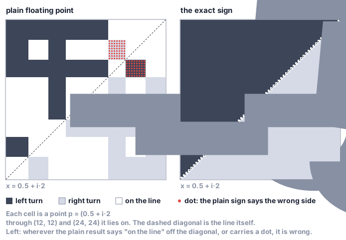
Both kinds of error hurt the hull. A false “on the line” is not a left turn, so when the turn is really left, the chain drops a point that is a real corner, and a point ends up outside the fence. A wrong side keeps a point that makes a dent, or drops a corner.
The library’s orient2d keeps the speed of the plain version and the answer of the exact one. It computes the plain value first, and trusts its sign only when the value is farther from zero than rounding could have moved it, by Shewchuk’s error bound [50, Sec. 4]. Otherwise it computes the same determinant again in exact fractions. Away from a line the plain sign clears the bound and is used as it is. Only near a line is the exact step paid for. The library’s Rust does the second step with Shewchuk’s adaptive arithmetic instead of fractions. Its floats can overflow or underflow, so where a step could, it answers “cannot decide” rather than guess, and every input whose coordinates are zero or of size between \(2^{-400}\) and \(2^{500}\) is always decided.
4.15.3 Why random shadows keep a distance
A place like this one claimed that about \(\log n / \varepsilon^2\) random directions, times a constant, keep every distance among \(n\) points within a factor of \(1 \pm \varepsilon\), with high probability. Here is the proof for one pair of points, and then for all of them, with the bell-curve directions of Indyk and Motwani and the steps of Dasgupta and Gupta [13], [16, Lemma 7].
Take \(k\) random directions \(r_1, \ldots, r_k\), each coordinate drawn from the bell curve, the standard normal distribution, all independently. Each \(r_i\) points in a random direction, as the directions of Figure 4.14 do. Its length only sets the scale, and the next step shows the scale comes out right. A point \(v\)’s shadow along \(r_i\) is the dot product \(s_i = r_i \cdot v\), and its new description is \(f(v) = (s_1, \ldots, s_k) / \sqrt{k}\), as the library’s projection computes it. In this appendix a shadow is the plain dot product, the shadow of A place like this one times the direction’s length, which is about 10 for a hundred numbers, so \(s_i^2\) already carries that section’s “multiply by 100”. Dot products add, so \(f(u) - f(w) = f(u - w)\), and the distance between two shadows is the length of one vector’s shadow, \(v = u - w\). Scaling \(v\) scales \(f(v)\) by the same factor, so take \(v\) of length 1.
Right on average. \(s_i = \sum_j r_{ij} v_j\) is a sum of independent bell-curve numbers, each scaled by \(v_j\), and such a sum is again a bell-curve number whose variance is the sum of the squared scales: \(\sum_j v_j^2 = 1\). So each \(s_i^2\) averages 1, and
\[ |f(v)|^2 = \frac{1}{k} \sum_{i=1}^{k} s_i^2 = \frac{X}{k} \]
averages 1 too. The question is how far \(X\) strays from \(k\).
Rarely far off. For a bell-curve number \(s\) and any \(t < 1/2\), the average of \(e^{t s^2}\) is \(1/\sqrt{1 - 2t}\), a standard integral. The \(s_i\) are independent, so the average of \(e^{tX}\) is \((1 - 2t)^{-k/2}\). A number that is never negative exceeds \(m\) times its average with probability at most \(1/m\) (Markov’s inequality). Apply it to \(e^{tX}\), which is never negative. For \(t > 0\), \(X \ge (1 + \varepsilon) k\) exactly when \(e^{tX} \ge e^{t (1 + \varepsilon) k}\), so
\[ P\big(X \ge (1 + \varepsilon) k\big) \le \frac{(1 - 2t)^{-k/2}}{e^{t (1 + \varepsilon) k}} . \]
The choice \(t = \varepsilon / (2(1 + \varepsilon))\) makes the right side \(\big((1 + \varepsilon) e^{-\varepsilon}\big)^{k/2}\), and since \(\ln(1 + \varepsilon) \le \varepsilon - \varepsilon^2/2 + \varepsilon^3/3\), that is at most \(e^{-k(\varepsilon^2/4 - \varepsilon^3/6)}\). The same steps with \(e^{-tX}\), whose average for one \(s\) is \(1/\sqrt{1 + 2t}\), and \(t = \varepsilon / (2(1 - \varepsilon))\) give \(P\big(X \le (1 - \varepsilon) k\big) \le \big((1 - \varepsilon) e^{\varepsilon}\big)^{k/2}\), and since \(\ln(1 - \varepsilon) \le -\varepsilon - \varepsilon^2/2\), that is at most \(e^{-k \varepsilon^2 / 4}\). For \(\varepsilon \le 1/2\) both are at most \(e^{-k\varepsilon^2/6}\), so
\[ P\Big(|f(v)|^2 \notin \big[1 - \varepsilon,\; 1 + \varepsilon\big]\Big) \;\le\; 2\, e^{-k \varepsilon^2 / 6} . \]
When the squared length stays inside \(1 \pm \varepsilon\), the length itself stays inside it too. That settles one pair.
All the pairs. \(n\) points make fewer than \(n^2/2\) pairs. The chance that at least one of them strays is at most the sum of their chances, the union bound, so at most \(n^2 e^{-k\varepsilon^2/6}\). With \(k \ge 18 \ln n / \varepsilon^2\) that is at most \(1/n\). The count of directions depends on \(n\) and \(\varepsilon\), and not on how many numbers the points started with. For a million points kept within 10%, these constants ask for about 25,000 directions. The two bounds above, before they were merged into one, ask for about 18,000. Either way it is tens of thousands.
4.15.4 A grid on a line
p-stable LSH
SimHash measures angle. For straight-line distance, LSH uses a different hash. Draw a random direction \(a\), each coordinate from the bell curve, a random offset \(b\) between 0 and \(w\), and cut the line into cells of width \(w\). A point’s cell is
\[ \Big\lfloor \frac{a \cdot v + b}{w} \Big\rfloor , \]
the cell its shadow falls in [18, Sec. 3.2]. With \(a = (1, 2)\), \(b = 0.5\) and \(w = 4\), the points \((3, 1)\) and \((2, 2)\) have shadows 5 and 6 and share cell 1, and \((1, 4)\), with shadow 9, lands in cell 2.
Two points in one cell have shadows less than \(w\) apart.5 The reverse fails. Two near points can sit on either side of a cell’s edge, and the random offset is what makes that a matter of chance. Shadows \(t\) apart, with \(t < w\), are split by an edge with probability \(t / w\), so they share a cell with probability \(1 - t/w\).
How far apart are the shadows? By the same fact as in the last proof, the shadow of \(u - v\) is a bell-curve number scaled by the distance \(c = |u - v|\). That is what stable means here. So the chance that \(u\) and \(v\) share a cell is the average, over a bell-curve number \(Z\), of \(\max(0,\, 1 - c|Z|/w)\). It falls as \(c\) grows, so near points share a cell more often than far ones, which is all LSH asks of a hash. From there the frame is SimHash’s: \(K\) cells make a key, \(L\) tables give second chances, and every candidate is measured exactly.
On GloVe, over the first 1,000 questions, the best setting of this hash that the library measured reached recall 0.843, at less than half the scan’s speed.
In the companion library’s Lean,
time_queryM_leinlean/AlgoDesign/Geometry/RangeTree/proves this for the walk as written, counting its steps one by one, at most \(2\lceil \log_2 n \rceil + k + 1\) for \(k\) keys reported.↩︎The measured numbers in the rest of the chapter come from a standard set of word embeddings, GloVe [6]: 1,183,514 words, 100 numbers each, with 10,000 test questions and their true ten nearest neighbors, as packaged by ann-benchmarks [7]. Like the cafés, they are compared by angle, every list scaled to length 1. The cafés stay a story. No number below was measured on them.↩︎
Rounds and numbers from one run of the Python bench, hidden seeds 101, 202 and 303 in both families, 10,000 places and 100 questions each. Practice numbers on seeds 1, 2 and 3. The same AI wrote both rounds, given only the bench and each round’s brief, the second with the judge’s report on the first. The chapter’s structures had their settings picked on the practice seeds.↩︎
In the library’s Lean,
far_side_bound,far_side_bound_leftandboxSqDist_leinKDTree/Prune.lean.↩︎In the library’s Lean,
pStableKey_eqinLSH/Families.lean.↩︎