2 Search
I leave to the various futures (not to all) my garden of forking paths.
Jorge Luis Borges, “The Garden of Forking Paths” (1941), trans. Donald A. Yates
Dude, where’s my car?
Dude, Where’s My Car? (film, 2000)
2.1 Where did I put my keys?
Your keys could be anywhere in the apartment. You check the couch. Nothing. You check the counter. Nothing. You’re checking at random, and each failed check tells you nothing about where to look next: the couch crossed off, the counter is no better a guess than the drawer. You’re just crossing places off a list, hoping the next one is it.
Now imagine a different life: every time you come home, you drop your keys on the same hook by the door. Finding them stops being a search at all: you reach for the hook and they’re there. You spent a little effort once, putting up the hook and using it every time, and that effort paid for every search since. The win moved out of the moment of searching and into the organizing you did ahead of time.
Now say you don’t just have one key. You carry a whole keyring: house, mailbox, garage, office, and half a dozen more you’ve picked up over the years, each one stamped with a number so you can tell them apart at a glance. Lose track of which is which, and finding key 12 means the same thing the couch and the counter meant a moment ago: checking each key in turn, with no way to skip ahead, because nothing about the order they’re threaded onto the ring tells you anything about where 12 might be.
So put them in order, low number to high, all the way around the ring. Now something changes. Hunting for key 12, you can glance at where you’d expect it and land close, instead of starting from one end and working through every key before it. Order turns “check everything” into “check nearby.”
But that order has to be paid for somewhere, and it’s paid for the moment you try to change it. Say a new key, 47, needs to go in, and it belongs squeezed between 46 and 48. There’s no gap sitting there waiting for it. Every key after 47 has to slide over one spot to make room, and the key after that, and the one after that, all the way around the ring. Fast to find, once it’s sorted. Painful to change, every time it isn’t.
That tension is the problem this chapter works through: a short ladder of ideas, each one fixing what broke in the one before it. It runs from checking a drawer at a time up through the structures that quietly hold the indexes of every database and filesystem you’ve ever used, and then one step further, to what those give up when the writes start arriving faster than the reads.
2.2 Checking one place at a time
Sequential search
That apartment search from before (couch, then counter, then wherever else) has a name: sequential search. You look at one place. Nothing there? Move to the next one, no wiser than when you started. In the worst case you check every spot before you find the keys or run out of places to look.
That worst case is the price, and the price is the reason to name it at all. A hundred places to look means up to a hundred checks. A keyring of a thousand keys in no particular order means up to a thousand checks to turn up key 12. Double the number of places and you double the work, one for one. And the worst case is common: it comes up every time the thing you want isn’t there at all, because being sure it’s missing means looking everywhere.
Sequential search is honest work, but it never gets smarter as it goes. That’s the baseline every design after it gets measured against.
Watch it on an actual few keys. Say the ring holds four so far, threaded on in whatever order they arrived: 20, 5, 30, 12, and you’re checking whether 30 is already there before adding a duplicate. Start at the first key: 20, no match. Next: 5, no match. Next: 30, found, after three checks. Now check for 8, a key that was never added at all: 20, then 5, then 30, then 12, and you are back where you started, having been all the way round. Four checks, one for every key on the ring, before you can be sure 8 isn’t there. That’s the worst case in miniature.
Nothing shortcuts a miss. Being sure a key isn’t on the ring means every key that is there has to be compared against it and rejected; skip even one and it might have been the match. So a miss costs exactly N checks on a ring of N keys, no fewer. So sequential search costs at most N compares [1]. Building the ring this way pays that cost on every insert too, since checking for a duplicate before adding a new key is itself a full search: adding N keys one at a time, each check costing one more than the last (0, 1, 2, …, N−1 keys already there to compare against), totals \(0+1+2+\cdots+(N-1) = \frac{N(N-1)}{2}\). Building a ring of N keys this way costs about \(N^2/2\) compares overall, not N.
That quadratic bill, about \(N^2/2\) compares to build a ring of \(N\) keys, gets ugly fast, and it gets ugly right where the keyring stops being able to hold the problem at all. Nobody carries half a million keys. Plenty of real collections are that size and far past it, and they are all around you: the account numbers a bank keeps, the parcels a delivery network is holding somewhere right now, the photos on your phone.
So take half a million of anything, arriving one at a time, each arrival checked against everything already stored to be sure it isn’t a duplicate. That is over \(10^{11}\) comparisons to build the collection once. Ten times as many items, still an ordinary size for a real system, and it’s over \(10^{13}\). A hundred times, and it passes \(10^{15}\).
Better code would not shrink that bill. It is the honest price of checking one at a time, and it is why nothing at that scale is built this way. Everything after this section is an attempt to stop paying it.
2.3 An orderly key ring
Sorted array and binary search
Now put your whole keyring in order and use that order on purpose: a keyring laid out in order is what a programmer calls a sorted array.
One thing has to change first. A ring has no ends. Keep the keys threaded on it and there is no middle to glance at, because every key has a key on either side of it, all the way around. So take the ring off and lay the keys flat in a row, first to last. That is the first thing this chapter borrowed from the world and then quietly changed about it, and it will not be the last: the everyday picture gets you to the idea, and then the idea needs something the picture didn’t have.
Say you’re hunting for key 12 on a keyring of a thousand keys, sorted low to high. Checking one at a time from the start still means up to a thousand checks in the worst case. Being sorted has to buy you something faster than that. Before reading on, find a way to use the order to cut the work down, and see how far you can cut it.
Two or three minutes, on fifteen keys you write down. You’re done when you can say how many checks your method needs in the worst case, even if the answer is a guess.
2.3.1 Binary search
Say you’re hunting for key 12. Don’t start at one end and count through. Glance at the key sitting in the middle of the row. If it’s key 15, key 12 must be in the lower half, so throw out the whole upper half in one move; if it’s key 8, throw out the lower half instead. Either way, one glance drops half the row from consideration. That’s binary search: check the middle, then go left or right depending on what you see, and repeat on whatever’s left. What makes that safe to do is an invariant: a property that is true again every time a step finishes, however things look part-way through one. Here the invariant is that the key, if it’s here at all, is always somewhere inside the stretch still under consideration. Every glance preserves that, which is why throwing away the other half can never lose anything.
Here’s what that actually looks like on a real row. Say the row holds fifteen keys, sorted: 2, 5, 8, 11, 14, 17, 20, 23, 26, 29, 32, 35, 38, 41, 44, and you’re hunting for 38. Glance at the middle key, 23. 38 is larger, so the whole left half (seven keys) is gone in one glance. Look at the middle of what’s left: 35. Still larger, so the next few keys are gone too. Middle of what’s left now: 41. This time 38 is smaller, so 41 and everything past it goes. One key left: 38. Found: four glances, on a row of fifteen.

That’s the shape of the payoff: doubling the row’s length doesn’t double the checks you need. It adds about one more. A row of 4 keys takes about three checks; a row of a thousand takes about ten. That slow, one-more-check growth as the row doubles is what the term \(\log_2 n\) labels. From here on this chapter writes it \(\lg n\), which is the usual shorthand for a logarithm in base 2 and means the same thing. You don’t need the formula to feel it: you already felt it in the four glances above.
A reader who just wants the idea can stop here and move on. The rest of this chapter builds on “halving beats checking one at a time,” nothing more. What follows in the rest of this section is the proof that the halving really does stop where it claims to, the general rule this is one instance of, and what to do when you don’t even know where the far end of the row is. The bill for the trick comes due right after that.
Let \(C(N)\) be the worst-case number of glances on a row of \(N\) keys. One glance either lands on the key or throws away half the row, leaving a search of at most \(\lfloor N/2\rfloor\) keys, so \(C(N) \le C(\lfloor N/2\rfloor)+1\), with \(C(0)=0\) [1]. Unrolling that recurrence for \(N=2^n-1\) gives \(C(N) \le n = \lg(N+1)\); the general case, any \(N\), rounds up to \(C(N) \le \lceil\lg(N+1)\rceil\). That’s the whole proof behind “about one more glance every time the row doubles” from the fifteen-key trace above.
2.3.2 Why it is logarithmic
One thing about that shape is worth separating out, because it is the actual reason binary search is \(O(\log n)\), and it is not “halving”. It is cutting by a fixed fraction rather than a fixed amount.
Guess before reading on: throw away a third of what’s left at every glance instead of half, and is the search still logarithmic? Throw away ten keys per glance instead, and is it?
Throw away a third of what’s left every step and you are still logarithmic: a different base, the same shape. Throw away a fixed number of keys per step, ten at a time no matter how long the row has grown, and you are \(O(n)\) however large you make that ten [2]. Sequential search is the extreme case: it discards exactly one key per glance. A constant amount, not a fraction, which is the whole of why it is linear and binary search isn’t.
On the same half-million-account row from before, the gap between the two ideas is stark: binary search needs at most \(\lceil\lg(500{,}001)\rceil = 19\) glances to find any account, worst case. Sequential search needed up to half a million, on the exact same row. Nineteen against half a million: that is what never needing to look at most of the row buys.
2.3.3 Galloping search
Binary search does assume something sequential search never needed: knowing where the far end of the row is, so it can jump straight to the middle of what’s left. If keys keep arriving and nobody’s counted them, there’s no middle to jump to. Galloping search handles that case: probe outward at doubling distances, 1, then 2, then 4, then 8 keys past the start, until a probe overshoots the target, then binary-search inside just that last doubled bracket. Finding a key at position \(p\) this way costs about \(2\lg p\) glances total [3]. That is worse than plain binary search, by a small constant factor. What it buys is that it never had to know how long the row was. That matters whenever one glance is expensive enough that a wrong guess really costs you: a network round trip, a disk seek, a physical measurement, rather than a free comparison.
2.3.4 Insertion means shoving
Insertion into a sorted array
Sorted order bought you fast finding. It didn’t come free, and the bill arrives the first time anything changes.
Take the same fifteen-key row: 2, 5, 8, 11, 14, 17, 20, 23, 26, 29, 32, 35, 38, 41, 44. Add key 12. Finding where it goes is the trick you just learned, and it is cheap: four glances put it between 11 and 14. Now actually put it there. There is no gap between 11 and 14: sorted keys packed into consecutive slots leave none. So 14 shifts one slot along, and to make room for 14, 17 shifts, and 20, and 23, and every remaining key to the end of the row. Eleven keys move so that one key can arrive.
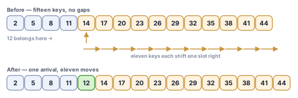
Watch that gap open up as the collection grows, because it opens fast. Half a million keys kept as one sorted row: 19 glances to decide where a new one goes, then a quarter of a million keys moved, on average, to make room for it. Thirteen thousand times more work putting the key in than working out where it belonged.
Design a way to store keys that keeps binary search’s fast lookup but doesn’t force every insert to shove half the row aside. Before reading on, sketch how you’d do it, even roughly.
Five minutes and one drawing. A sketch that doesn’t quite work is the right outcome here: what matters is that you’ve felt why “keep it sorted” and “don’t move anything” pull against each other.
Why does putting a key in cost so much? State it precisely, because the next structure is built to undo it. The keys don’t merely sit in order; their order is their position. Key 12’s slot is nothing but a count of how many keys are smaller than it, and that count is its address. Rank and position are the same fact written twice, so nothing can change its rank without changing its address, and nothing can change its address without displacing whatever was living there.
So the fast lookup was never free. It was paid for by tying every key’s rank to a fixed spot in the row. What if a key’s place in line didn’t have to be its place in memory?
The failure has a name worth keeping, because it recurs far outside this chapter: one-dimensional crowding. Lay things out along a line and a newcomer can only make room by shoving everybody else aside. The cure, every time it turns up, is the same: find a second direction to grow into.
2.4 Escaping the line
Binary search tree
Picture a different way to store the keyring: a branching arrangement of hooks. Each hook holds a key, and under each hook there is room for two more, one down and to the left, one down and to the right. Those can grow two more the same way, and so on down.
That hook has a name, and it is worth using from the start, because it is the name everyone else uses: a node. Every library’s documentation, every answer you will ever get from a search or a model calls it that, and so does this book’s companion library in all three of its languages. Keep the hook as the picture in your head. Say node out loud. The first one, the one everything else hangs beneath, is the root.
That’s a binary search tree: a key sits on a node, and the node can point to two smaller branching arrangements hanging under it, one on each side. A key’s place is no longer a slot you count to. It’s what the key hangs from.
The rest of the family comes off the same picture, and the words are everyone’s. The two nodes hanging directly under a node are its children, and it is their parent. Two children of the same parent are siblings. A node with nothing hanging under it is a leaf. Any node, taken together with everything hanging beneath it, is a subtree. Nothing here is deeper than the picture: a leaf is a hook with nothing on it yet.
That one change is what buys back the cost of the shoving, and it’s worth being exact about why. A row is a line. One direction, and the only free space on a line is at its end. To put a key in the middle of one you have to make room, and the only way to make room in a line is to push everybody along. There is no other move available to you.
A branching arrangement isn’t a line. It grows in a second direction, downward, and that direction never runs out. Count the empty spots and the difference is exact: a row holding \(n\) keys has one, its end. A branching arrangement holding \(n\) nodes has \(n + 1\). One dangling under every side that nothing hangs from yet: \(n\) nodes offer \(2n\) sides, every node but the root uses up one of them, and \(2n - (n - 1) = n + 1\) are left. Hanging a key fills one of those empty spots and leaves two new ones behind it. The room is already there, at the bottom, waiting, which is the reason nothing has to move to make it.
2.4.1 Order and duplicates
One rule keeps the whole arrangement searchable, and it’s the only rule it needs: everything on the left side of a node is smaller than that node’s key, and everything on the right side is larger.
\[\text{left} < \text{node} < \text{right}\]
Mind the word everything: the rule is about whole sides, not only a node’s two children. Draw this by hand: 50 at the top, 25 hanging on its left, and 60 hanging on the right of 25. Every parent and child look fine together, yet 60 sits on 50’s left side, and a search for 60 turns right at 50 and never finds it.
Read that rule twice, because both signs are strict, and that leaves a gap in it. It says where a smaller key goes and where a larger key goes. It says nothing about a key equal to the one on the node.
This chapter’s answer is the simple one: no duplicates. Hanging 50 on an arrangement that already holds a 50 does nothing at all, and the code below says so at its first comparison, reporting back that nothing was added. That is a choice, and I make it by default because it is the reversible one: every other way can be built on top of it later, and none of them can be taken back once the structure is already holding two of something.
Duplicates have to go somewhere, and there are only three places to put them.
The first loosens exactly one side of the rule, so equal keys have a settled home:
\[\text{left} \le \text{node} < \text{right}\]
Equal keys go left, always, and never right. Which side you pick doesn’t matter; picking a side does. Loosen both and a key equal to the node could sit on either, so a search has to try both, and one comparison stops throwing away half the arrangement, which was the entire reason for building it this way.
Even loosened on one side, it costs more than it looks. A search that finds the key can no longer stop, because another copy may be further down that same side, so search quietly turns into “find them all”. Deletion gets the same problem: removing a 50 is no longer the same instruction as removing the 50.
That is why the other two answers are usually better, and both keep the rule strict. Put a count on the node, if the copies are indistinguishable. Hang a list of items off it, if they aren’t. Either way the keys stay unique, the rule stays strict, and everything above it stays cheap.
Here is where that choice bites, and it bites quietly. Suppose you are logging events by timestamp and two of them land on the same millisecond. The second insert returns, no error is raised, nothing is logged, and the structure is one event short: the count is wrong and nothing anywhere says so. A structure that refuses duplicates loses the second one, and the only warning you get is the return value the code below hands back. That is the one place in this chapter where ignoring a returned value costs you data, which is why it is returned at all.
2.4.2 Search and insertion
Finding a key means starting at the root and asking one question at each stop: is what I want smaller or larger than the key on this node? Smaller sends you left, larger sends you right, and you keep stepping down one side or the other until you land on the key or run out of nodes. Each question throws away a whole side of the arrangement, everything hanging off it, without ever having to look at a single key on it.
Let’s watch it happen. Hang eight keys this way, one at a time, each one walking down from the first node until it finds empty air: 50 first, then 25 and 75 beside it, then 10 and 40 under 25, then 60 and 90 under 75, then 35 tucked under 40. That’s the whole insertion rule: walk down comparing, smaller left, larger right, and stop at the first empty spot, which is where the new node goes. No other key has to move. Here it is in code.
Code in this chapter is printed with a note beside each line or group of lines, and sometimes a small picture beside that. Read down the code first, on its own, then come back for the notes. Reading both columns at once is slower, not faster.
Now search that same arrangement for 35, a key that’s actually hanging there.
- At the root, 50: is 35 smaller or larger than 50? Smaller. Go left, to 25.
- At 25: is 35 smaller or larger than 25? Larger. Go right, to 40.
- At 40: is 35 smaller or larger than 40? Smaller. Go left, to 35.
- At 35: that’s the key. Found on the fourth comparison, having never once looked at 75, 60, 90, or 10: three comparisons chose a direction, and the fourth landed on it, counted the same way as the glances along the row.
The red path below traces those three steps down:
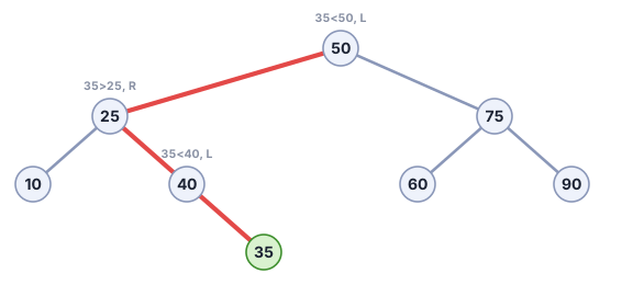
That’s the real difference from the keyring laid out in a row: a sorted array encodes order by where a key sits: its slot is its rank. A tree encodes order by what a key is next to: its place is just a pattern of left turns and right turns from the root. Hang new neighbors around a key and the key itself stays put; nothing has to shift down a row to make room for it.
2.4.3 Degenerate trees
But notice what no rule here forbids: nothing about this arrangement stops it from growing lopsided. Try it before reading on: start from an empty arrangement and hang 10, then 20, then 30, then 40, keys arriving already sorted, each one walking down from the root the same way as before. Sketch the shape you get, then check it step by step.
- Hang 10 first. No nodes yet, so 10 becomes the root.
- Hang 20. Start at 10: is 20 smaller or larger than 10? Larger, go right, and there’s no node there, so 20 hangs on the right side of 10.
- Hang 30. Start at 10: larger, go right, to 20. At 20: larger again, go right, empty, so 30 hangs on the right side of 20.
- Hang 40. Start at 10: larger, right, to 20. At 20: larger, right, to 30. At 30: larger, right, empty, so 40 hangs on the right side of 30.
Every key lands on the right side of the one before it, because every new key is always the largest so far. It never branches at all. It just grows into one long line down the right side:
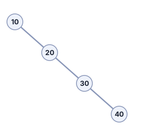
Look at what that picture actually is. The second direction was the entire point of moving off the row, and this arrangement has thrown it away: it uses one direction, like a line, and every key sits after the one before it, like a row. It is a row again, wearing nodes, and not a sorted row you can halve: its lookups cost what checking one place at a time costs.
Try it yourself: step through the same build, or hang and search your own keys:
But this freedom has a price, and that line is it. Searching this arrangement for 40 means walking past 10, then 20, then 30, one at a time. No question ever throws away a whole side, because there never is a side to throw away. That’s the same problem from the very start of the chapter, wearing a different shape: sequential search, with a tree’s name on it.
2.4.4 Order queries
Insert and search aren’t the only things this shape buys. The same left/right walk answers a handful of other questions almost for free. min and max just walk all the way left, or all the way right, and stop: the smallest and largest keys are the leftmost and rightmost nodes, no comparisons needed once you’re already walking that direction.
floor and ceiling are the next two. floor means the closest key at or below a target, and ceiling the closest at or above, and the target may not be in the tree at all, which is the whole reason you’d ask. They need one extra idea beyond the ordinary walk: keep the best candidate you have seen so far. For floor, a node at or below the target is a candidate, and the walk then goes right to look for a closer one; a node above the target is not, and the walk goes left. ceiling is the mirror image. When the walk runs out of nodes, whichever candidate survived is the answer. In the recursive version below there is no variable holding it: the candidate is node.key, kept on the way back out whenever the right side turned up nothing better:
rank (how many keys are smaller than this one) and select (which key sits at a given position) need one more thing neither min/max nor floor/ceiling do: every node has to know, kept up to date on every insert, how many keys its subtree holds, its own key included. With that one extra field, rank walks down the same way search does, and on every rightward step adds the size of the left subtree it passes plus one for the node it steps past, and on reaching the key, the size of that node’s left subtree; select walks down comparing a target position against the left subtree’s size instead of comparing keys. Every one of these costs exactly what search and insert already cost: one comparison per node, and as many nodes as the tree is tall. That number has a name worth fixing now, because everything from here on is about controlling it. A tree’s height is the number of steps down the longest walk from the root to a place where a node could hang but doesn’t. Counting to the empty spot rather than to the last node makes a single node a tree of height one; counting to the last node would make it zero. The difference doesn’t matter here, but your own hand-traces will be off by one if you mix the two counts.
Try three of these on the eight-key tree you built, before opening the answers: floor(45), rank(40), and select(3), counting select(0) as the smallest key.
floor(45) is 40. At 50, too big: go left. At 25, a candidate: go right. At 40, a better one: go right, and the walk runs out. The last candidate stands.
rank(40) is 3. At 50, go left and add nothing. At 25, go right and add 1 for the subtree holding 10, plus 1 for 25. At 40, the key: add 1 for the subtree holding 35. The three smaller keys are 10, 25 and 35.
select(3) is 40. At 50, the left subtree holds four keys and position 3 is among them: go left. At 25, the left subtree holds one key, so position 3 is past it and past 25: go right looking for position \(3 - 1 - 1 = 1\). At 40, the left subtree holds one key, exactly position 1’s worth: 40 is the answer.
The size field is one case of a move worth naming, because it is far more general than counting. A node can carry any summary of its subtree that is computed from its own key and its two children’s summaries: a count, a sum, a smallest value, a largest one. The one requirement is that combining summaries gives the same answer however the pieces are grouped, which is what associative means, because a walk down the tree meets its pieces in whatever grouping the tree’s shape happens to have. Let each account in the bank carry its balance, and let every node store the smallest balance in its subtree instead of its size. Two walks of the same kind, one down toward each end of a range, collect the summaries hanging between them and answer “which account numbered between these two has the lowest balance,” still at the cost of the height: a new question with no new structure. Nothing in that argument is about trees. Any quantity whose pieces combine associatively can be kept this way, which is why the same move turns up well outside search trees: running totals over an array are the flattest case of it, and summaries of a data stream computed on separate machines can be merged into one for the same reason.
2.4.5 Deletion
Deletion has three cases, and two of them are easy. A node with no children: unhook it, done. A node with one child: the child moves up into its place, and order still holds, because everything in that child’s subtree was already on the correct side of the parent above.
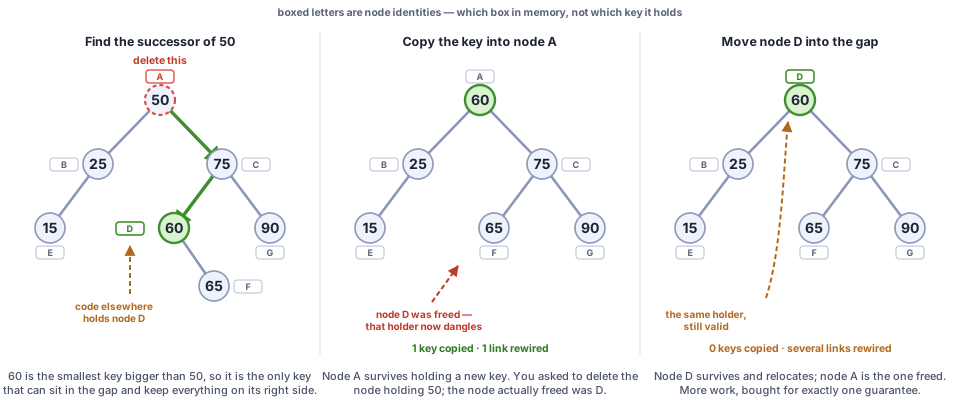
The third case is the real one: a node with two children. Pull it out and a gap opens that something must fill, and the two subtrees hanging beneath it both have to stay on their correct sides. Only two keys in the whole tree can sit in that gap: the smallest key bigger than the one leaving, or the largest key smaller than it. Take the bigger one. Every key in the left subtree is smaller than it, every remaining key on the right is bigger, so order survives. (The smaller one works just as well by the mirror argument. There is a reason to care which you pick, and it arrives at the end of this section.) That key is the deleted node’s successor, and you find it by walking right once and then left as far as you can go.
However the gap is then filled, and there are two ways, coming up below, the successor is easy to remove from where it was standing: being the leftmost thing in that subtree, it has no left child, so at most one child hangs off it and that child simply moves up: the one-child case you already know.
That is the binary search tree in one sentence: a tree is a row that grew a second direction, so nothing has to move, and it degenerates back into a row whenever the keys arrive already sorted. If that’s what you came for, you have it, and the next section is where the chapter fixes the degeneration. What’s left here is the choice between two ways of finishing a deletion and what a tree’s height averages out to when the keys arrive in random order.
There are two ways to put the successor in the gap, and they differ in which node survives; the keys come out the same.
Copy the key. This is Hibbard’s deletion [4]. In the figure’s tree, write 60 into the old node, then remove the successor’s own node by the one-child rule. One key copied, one link rewired. Simple and cheap.
One thing this is not: a chain. Having copied 60 upward, you do not then go and find 60’s own successor and copy that up too, and so on down to a leaf. The successor’s node has at most one child, so the ordinary one-child case finishes it in a single relink. Copying again would just be extra work for the same tree.
Move the node. Unhook the successor and put that node itself in the gap, re-pointing it at the dead node’s two subtrees. Nothing is copied; several links get rewired: noticeably more work than the first way.
So why pay? Not for speed. Because the first way deletes a different node than you asked it to. You asked to delete the node holding 50; what actually got freed was the node holding 60. If anything else in the program was holding that node (an iterator, an index, a cache) it is now holding something dead. Moving the node guarantees that deleting a node deletes that node and nothing else.
The preference has flipped over time. Copying was standard for decades, on the reasonable grounds that it is cheaper, and it is also the one that quietly bites. The major texts now teach moving the node instead [5], which is the trade this book keeps making: a guarantee is usually worth a little speed. I will not pretend to be neutral about that trade. Most of the expensive hours of my working life have gone on bugs of one shape: a structure that was fast almost always, and then failed on a day I did not choose, in a way that looked like something else.
Whether it matters to you comes down to whether anything outside the tree can hold a node. Where it can, identity is part of what you promised. The companion library moves the node in its Python and its Rust, and only the Python lets you feel why: it moves the node object, so a reference held elsewhere still points at a live key. The Rust hands out no node that outlives an update, so the question cannot be asked of it, and the Lean works on values alone, so it has no node to move.
Which leaves the question of whether the two deletions build different trees, and the answer depends on what you call the tree. Read it as values, keys in a shape, and they build the same tree: the library proves that in Lean and its tests check it on every small tree. Read it as nodes, the objects and the pointers that lead to them, and they build different trees, because a different node sits in the gap. A test that looks only at keys and shape cannot tell the two apart. Only a test that holds on to a node can.
One practical warning. Always taking the successor, never the predecessor, is lopsided, and over long runs of delete-and-insert that lopsidedness accumulates: paths get longer than they are in a tree built by random insertions alone. Alternating between successor and predecessor removes the effect [6]. The degradation is \(\Theta(\sqrt{N})\) under a restricted model where every deletion is immediately followed by an insertion [7]; for ordinary mixed workloads that figure is widely observed rather than proved [8].
Draw an eight-key tree. Delete a key with two children, by hand. Say out loud, before you move anything, which two keys are allowed to fill the gap, why no other key would do, and which one this chapter picks. Then check the result reads in the same sorted order as before, minus the key you removed.
2.4.6 Average height
None of this changes the headline promise this tree was built around: search and insert cost time proportional to height, and nothing more. What height actually comes out to, averaged over many random insertions rather than assumed worst case, is itself a proved result: a tree built from N keys arriving in random order costs about \(2\ln N \approx 1.39\lg N\) compares on average for a search or insert, and its height converges to about \(2.99\lg N\) [1]: the height result in particular took until 1986 to pin down exactly, long after the average-cost result itself was understood [9].
Those averages are known exactly, not merely to within a constant.
None of this box is derived in front of you; the derivations are real work and belong elsewhere. But three different things are going on here, and they are worth keeping apart, because “proved” is doing different amounts of work in each.
Writing \(H_N\) for \(1 + \frac{1}{2} + \cdots + \frac{1}{N}\), building the tree from \(N\) random keys costs \(2(N+1)(H_{N+1} - 1) - 2N\) comparisons on average [9], and a successful search costs \(2(1 + \frac{1}{N})H_N - 3\): the build cost divided by \(N\), plus one.
Both come from the same move. Average over every insertion order and the question turns into a recurrence: with \(N+1\) keys, you pay \(N\) at the root, then the average cost of the two piles the root splits the keys into. Getting to that recurrence is where the “random order” assumption is spent. That step is Sedgewick and Flajolet’s, and you’re taking it on their word. Turning the recurrence into the formulas above is algebra, and that part is machine-checked on every build.
Worth knowing which is which. A proof checks the step you wrote down. It says nothing about whether you wrote down the right thing, and for average-case results, that’s the step that usually breaks.
The height constant is shakier again. It’s the number \(c \approx 4.31107\) solving \(c\ln(2e/c) = 1\). What’s checked is only that some root exists between \(2\) and \(2e\). That it’s near \(4.31107\), and that there’s only one: Sedgewick and Flajolet again, on their authority.
So: two formulas whose algebra is checked, one constant you’re trusting. Nothing later in the chapter depends on any of them.
One more question this tree doesn’t answer at all: what if some keys get looked up far more often than others? There is a best possible tree for a known set of access frequencies, and it is not the shortest one. Finding it is a real and solved problem, and it is waiting in the frontier map at the end of this chapter rather than here, because nothing between here and the end of the chapter depends on it.
That’s everything the plain tree has to offer, the win and the way it breaks. Before climbing to the fix, name what has actually been under construction all along.
2.5 What is this all about?
The ordered dictionary (dynamic set)
Step back for a second from keys and nodes. What this chapter has been building, one structure at a time, is one abstraction wearing different clothes: an ordered dictionary, sometimes just called a dynamic set. Underneath the couches and counters and keyrings, every design so far answers the same short list of questions about a changing collection of ordered items:
- Is this one in here? (
search) - Put a new one in. (
insert) - Take one out. (
delete) - Which one is smallest, or largest? (
min/max) - Which item sits just below, or just above, a value: even when that value isn’t in the collection at all? (
floor/ceiling) - Treating the collection as a sorted list without ever sorting it: which position does this item hold, and which item sits at this position? (
rank/select)
Numbered keys made those questions easy to picture, but they aren’t about keys. Swap in the account numbers a bank holds, and every question on that list is one its systems answer continuously. search is “does this account exist.” insert and delete are opening and closing one. min and max find the lowest and highest account numbers still open. floor and ceiling answer “the nearest existing account number to this one,” which is what you need when the number you were given is slightly wrong. And rank and select answer “how many open accounts have a smaller number than this one” and “which one is the ten-thousandth in number order.” None of that is exotic. It is the same short list any system that keeps things in order eventually has to answer, whether the things are keys, accounts, parcels or messages.
Each structure in this chapter answers that short list differently, and the differences are the story:
| Structure | Rough cost shape | What it buys | What it costs |
|---|---|---|---|
| Sequential search | \(O(n)\), every operation | Nothing to build or maintain | No question is ever cheap |
| Sorted array, binary search | \(O(\log n)\) search, \(O(n)\) insert | Fast lookup | Painful to change |
| Binary search tree | \(O(h)\), height unbounded | Cheap insert, nothing shifts | Can degrade toward \(O(n)\) |
Three structures, and the pattern is already visible in the last two columns: whatever a structure wins in one column, it pays for in the other. There is no row that wins both, and there will not be one. Every design still ahead is another line in that ledger, bought the same way, and none of them breaks the rule.
Which puts the plain tree’s row in focus, because that is where this chapter currently stands: inserts that shift nothing, bought with a height that nobody is guarding. So the tree needs a rule that stops it from leaning too far, without being expensive to maintain.
Before reading on, try to invent a rule of your own: some small, local check the tree could make after every insert that would stop it from growing into one long line, without re-checking the whole tree from scratch each time. What’s the cheapest signal you can think of that a tree has tipped too far?
Ten minutes. This one is genuinely hard, it took the field years, so the bar is not a working rule. The standard is one candidate signal and one reason it might be too expensive to keep up to date.
2.5.1 What “balanced” is allowed to mean
Balance conditions
Whatever rule you came up with, it was a rule about shape, and the word covering all such rules is “balanced”. Pin that word down: it names at least four different promises, they are not equally strong, and the design question from here on is which of them is worth its price.
Measure a tree’s height the way this chapter already has: the number of steps down the longest walk from the root to a place where a node could hang but doesn’t. That is the number every promise below is trying to control.
Perfectly balanced. Every such walk is the same length: not roughly, exactly. The strongest thing you could ask for, and a binary tree can only manage it at all when \(n\) is one less than a power of two; for every other count there is simply no binary shape with all its walks equal, and the best available is walks that differ by one. Even that much is out of reach under a stream of inserts: hang one more key and some walk gets longer, and there is no local repair that puts the shape right again without sometimes rebuilding a large part of the tree. Worth naming anyway, because it is not hopeless everywhere: the B-tree later in this chapter keeps the exact version of this promise, for any \(n\), by letting a node grow wider instead of letting the tree grow taller.
Height-balanced at every node. At every node, the heights of the two sides differ by at most one. This is the AVL tree’s rule [10], the first invariant anyone managed to maintain on the spot after every insert, and it holds the tree to roughly \(1.44\lg n\): closer to perfect than anything else here. The phrase at every node is load-bearing and easy to weaken by accident: ask only that the two sides of the first node match, and you have asked for nothing at all, because both sides can still be the long lines a balanced tree is meant to outlaw.
Balanced, loosely. No walk down is more than about twice as long as any other. That’s the promise the red-black tree keeps, and the word “balanced” without qualification usually means this one: not a fixed shape, just height held to within a constant factor of \(\lg n\), which is all \(O(\log n)\) ever asked for.
Weight-balanced. Same idea, counted in keys rather than in steps: at every node, neither side holds more than some fixed fraction of the keys below it [11]. It buys the same kind of height bound, and it is the one notion of the four that also tells you something directly about rank and select, since it is already counting.
If you are allowed to stop the world, one linear pass of rotations will rebuild any binary search tree into a perfectly balanced one, in time proportional to the number of keys: the Day-Stout-Warren algorithm. That is not the problem here. The problem is staying balanced while the updates keep arriving.
So: which one? Every rule after the first keeps height proportional to \(\lg n\), so all of them sit in the same complexity class, and choosing between them is choosing a constant factor. AVL wins that comparison outright, \(1.44\lg n\) against roughly \(2\lg n\), and a tree that is asked far more often than it is changed is a real case for paying AVL’s price. But what differs between these rules by much more than a constant is how much code it takes to keep one true, and how many distinct broken shapes a repair has to recognize.
I teach the looser rule, and that is a preference rather than a result: a tighter tree that I get wrong is worth less than a slightly taller one I can hold in my head. It is also what this book builds on. The left-leaning red-black tree maintains it with three repair moves and one extra bit per link, and the B-tree carries the same idea further, letting a node hold more than one key. AVL is not developed here. Its rotations are the same two moves you are about to meet, driven by a stricter test, and Drozdek develops it in full [12].
One more thing, if you have met red-black trees before or expect to meet them elsewhere. The version this chapter builds is the left-leaning one, not the standard one [5], [13]. The difference is two extra promises, and the appendix at the end of this chapter is the translation: what the standard rules are, why they are the rules, and the single shape the two trees disagree about. Read the next section first. The appendix then takes about twenty minutes instead of an afternoon, because it is the same encoding with those two restrictions lifted.
2.6 Sticky red links
Left-leaning red-black tree (LLRB)
2.6.1 Red links and the five rules
Give every link one extra bit: red or black. Not the node, the link, the connection running from a node down to whatever hangs on its left or right. That single bit is a promise the structure makes and keeps on every step. It is the invariant idea again, put to a new job: pay a little on every insert, so every lookup after it stays cheap.
Picture it on the smallest possible case first: hang key 20, then hang 10 underneath it, off to the left. The link joining them is the one that just got colored: red, and leaning left.
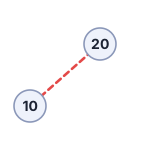
That’s the picture the rules below are actually about. Remember it.
Before the rules, one sentence that makes all of them follow instead of having to be remembered.
A red link isn’t really a link. It’s glue. Two nodes joined by a red link are one node that happens to hold two keys. Look at the picture again: 10 and 20 are drawn as two nodes, but the red link between them says treat us as one. Black links are the real steps down the tree. Red links are joinery inside a node.
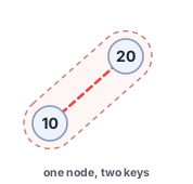
Read that way, the rules below stop being rules and start being consequences. A node holds one key or two and never three, so no node may have two red links touching it. The two keys in a node always sit the same way round, so a red link always leans left. And “every path crosses the same number of black links” turns into something much plainer than it sounds: since only black links are real steps down, every leaf sits at exactly the same depth. The tree is perfectly balanced. It just doesn’t look it, because some of its nodes are drawn as two.
Two different heights are in play from here on, so separate them now rather than tripping over them later. Count only black links and every path is the same length, exactly: the tree’s black height. That is the perfect balance just claimed, and it is a statement about the tree as the glue picture shows it, nodes counted once. Count every link, red ones included, and the paths differ, because a path that passes through several two-key nodes takes an extra step inside each one. The second number is the one a lookup actually pays, and the rules below exist to keep it from drifting too far from the first.
Five rules make a valid tree. The keys are in order, as in any search tree. The top node is black. A red link always leans left, never right. No node ever has two red links touching it, not one on each side, and not one chained below the other. And every path from the root down to a spot where you’d fall off the tree crosses the same number of black links.
The last three are what bound the height: the second height, the one counting every link. Because red links can never chain, at most every other link on a path down the tree is red. Because the black count is the same everywhere, every path carries the same black backbone underneath. So the longest way down can never be more than roughly twice the shortest: a path of all black links in the best case, alternating black and red in the worst. The tree never grows more than roughly twice as tall as the best possible, and height stays bounded without anyone ever having to measure it.
The lean-left rule is what gives this structure its name: this is a red-black tree, specifically the left-leaning variant, LLRB for short, due to Sedgewick [1].
2.6.2 Insertion: rotations and color flips
Insertion still starts the same walk as before: compare left or right, node by node, until you fall off the tree, and hang the new key there. The only change is that the new node arrives attached by a red link. That red link can break one of the rules above, so on the way back up, node by node, toward the root, the tree checks itself and applies whichever of three small, local repairs the broken rule calls for:
- rotate left: a red link leans right. Rotate, and it leans left instead.
- rotate right: two red links lean left in a row, one chained right below the other, so the node in the middle has a red link coming in from above and another going out below. Rotate, and the pair becomes one node with a red link on both its left and right side.
- flip colors: a node has red links on both sides. Flip both to black, and send a single red link up to the node above it.
The third one is worth reading through the glue picture, because it isn’t really a repair. A node with red links on both sides is a node holding three keys, and a node may not hold three. So the middle key moves up into the node above and the outer two stay behind as nodes of their own. That is a split, and it is the same move a much larger structure later in this chapter is built entirely out of.
Each repair only touches a node and its immediate neighbors, and a handful of them, applied on the way back up, is always enough to restore every rule.
Watch it happen on an actual tree. Start empty, and hang five keys in this order: 10, 20, 30, 15, 5.
Hang 10: it’s the root, nothing to check. Hang 20: 20 is bigger than 10, so it goes on 10’s right, on the end of a new red link. Check the rules: that red link leans right. The lean-left rule, broken, which calls for rotate left at 10: 20 comes up to take 10’s old spot, and 10 drops down to hang off 20’s left side on a red link. One node, one red link, and it leans left now.
Hang 30: 30 is bigger than 20, so it goes on 20’s right, on another new red link. Now look at node 20: a red link on the left, to 10, and a red link on the right, to 30. The no-two-reds rule, broken: two reds touching the same node.
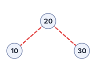
That’s what flip colors is for: turn both of 20’s links black, and send a single red link up to whatever node sits above 20. There is no node above 20, it’s the root, so that red link has nowhere to go, and the fix-up simply stops there. Three nodes, two black links, every rule holding.
Hang 15: 15 is smaller than 20, so go left to 10; 15 is bigger than 10, so it lands on 10’s right, on a red link. Leaning right again, the lean-left rule, broken, calling for rotate left at 10: 15 comes up to take 10’s old spot as 20’s left side, and 10 drops down to hang off 15’s left side on a red link.
Before reading on, hang 5 yourself: where does it land, which rule does it break, and which repair fires first?
Hang 5: 5 is smaller than 20 (left, to 15), smaller than 15 (left, to 10), smaller than 10: it lands on 10’s left, on a red link. On its own, that link is fine: it leans left. But look at what it sits under: 15’s link down to 10 is red, and now 10’s link down to 5 is red too, two red links in a row, both leaning left, one chained right below the other.
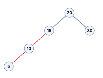
That’s the shape rotate right targets, so that repair fires at 15: 10 comes up to take 15’s old spot, and 15 drops down to hang off 10’s right side. Now 10 has a red link on its left, still to 5, and a red link on its right, to 15, just arrived. That’s the no-two-reds rule again, two reds touching one node, so the fix-up doesn’t stop at the rotation: flip colors fires right away, turning both of 10’s links black and sending a single red link up to 20, replacing what used to be a plain link down to 15’s old spot. Check node 20 once more: a red link on the left, a black link on the right, no two reds touching anywhere, and the fix-up is done.
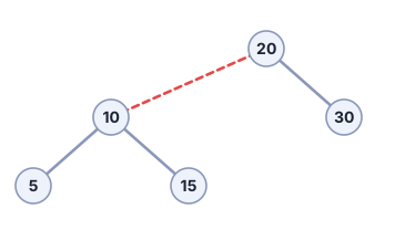
Try it yourself: step through the same five keys, or hang your own and watch the repairs fire:
Five keys, five repairs, and at no point did the tree touch more than a node and its immediate neighbors. Laid out as a ledger, one line per key hung:
| Hang | Repair that fired | What the tree looks like after |
|---|---|---|
| 10 | none | 10 alone |
| 20 | rotate left at 10 | 20, with 10 on a red link to its left |
| 30 | flip colors at 20 | 20, with 10 and 30 both black |
| 15 | rotate left at 10 | 20, with black 15 on the left and red 10 beneath it |
| 5 | rotate right at 15, then flip colors at 10 | 20, with red 10 carrying black 5 and 15, and black 30 |
Note the fourth line: hanging 15 needed a rotation, but the rotation happened to land the tree in a shape that broke nothing else, so the repair stopped there. And the fifth needed two repairs in a row, the second one triggered by what the first one produced. That is the whole promise being kept: pay a little, locally, on the way back up, every time, and the tree never has to re-examine anything it already fixed.
If that’s enough to see the shape of it (three small repairs, undoing whatever the last insert broke, node by node on the way back up) you have the left-leaning red-black tree, and you can skip ahead to the B-tree. The rest of this section is the code those three repairs actually compile down to, a short aside on the trade this version makes against the classic red-black tree, the 2-3 tree this one comes from, and then deletion, which needs one genuinely new idea.
Here h.red is the color of the link coming down into node h from whatever node is above it. Every node but the root has exactly one link coming down into it, so that link’s color can live in the node it leads to, and one field per node is enough. It is also why the code, and sometimes the prose, calls a node red: the link into it is red. fix_up runs on the way back up from every insert, checking the three conditions in order and applying whichever repair matches: exactly the three bullets above, nothing more.
An aside: the standard red-black tree [13] allows two shapes this version forbids: a red link leaning right, and a node with red links on both sides left in place, a node holding three keys, sometimes called a 4-node. Both need more case-handling to keep balanced. This version gives them up on purpose, in exchange for exactly three repair rules instead of a longer list.
Red links aren’t the only way to get a guarantee like this. The AVL tree named a few pages back reaches a better bound by insisting on a stricter rule at every node and paying for it in cases; the skip list waiting in this chapter’s frontier map reaches the same bound by not keeping a rule at all, and flipping coins instead.
2.6.3 Where LLRB actually comes from
2-3 tree
The glue picture was doing more work than it let on. There is a real structure standing behind it, and naming it turns every rule of LLRB from something to remember into something that could not have been otherwise. A 2-3 tree is a search tree whose nodes hold either one key or two, and never more, and whose leaves all sit at the same depth.
Two shapes, and only two. A 2-node holds one key and has two children, smaller on one side and larger on the other, an ordinary binary search tree node. A 3-node holds two keys and has three children: smaller than both, between them, larger than both. That third child is the one shape a 2-3 tree allows that a plain binary node can’t.
So how does a 3-node fit inside an ordinary node, which only has room for one key and two children? Split it: two nodes, one holding each key, joined by a link between them. Color that joining link red, marking that these two nodes are secretly one 3-node, pulled apart only because a plain node can’t hold two keys at once. Every other link (connecting genuinely separate 2-3 tree nodes) stays black. A 2-node needs no disguise: it’s already a plain node with only black links to its children.
Here is that translation on the tree you just built: the one the five keys made, a page ago.
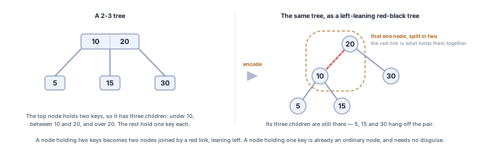
Compare the two sides key by key. They hold the same five keys, in the same order, with the same three subtrees hanging underneath. The right-hand picture is the left-hand picture, written down differently.
Which side does the pair lean on? Hang the second node down and right of the first and the red link leans right; down and left, and it leans left. Either encodes the exact same 3-node just as validly. A 2-3 tree doesn’t care which side its binary disguise leans on. LLRB just picks one side, left, and enforces it everywhere, purely so there’s one fewer shape to handle in every piece of code that walks the tree. Left-leaning is a convention, chosen for convenience.
But picking a side buys something beyond convenience, and it is the reason this section is worth reading. With the lean fixed, the translation runs both ways with no choices in it. Every 2-3 tree becomes exactly one left-leaning red-black tree, and every left-leaning red-black tree becomes exactly one 2-3 tree. Nothing is lost in either direction and nothing is ever decided along the way, which is what a mathematician would call a one-to-one correspondence. Allow the pair to lean either way, as the standard red-black tree does, and that stops being true: each two-key node then has two legal drawings, and the same 2-3 tree answers to more than one red-black tree.
It is a correspondence between trees at rest. Insertion keeps to it step for step: every insert into the left-leaning tree is the 2-3 tree’s insert, drawn in links. Deletion, later in this section, does not.
The payoff is that anything true on one side is now automatically true on the other. The rest of this section collects LLRB’s rules that way, rather than arguing them from scratch.
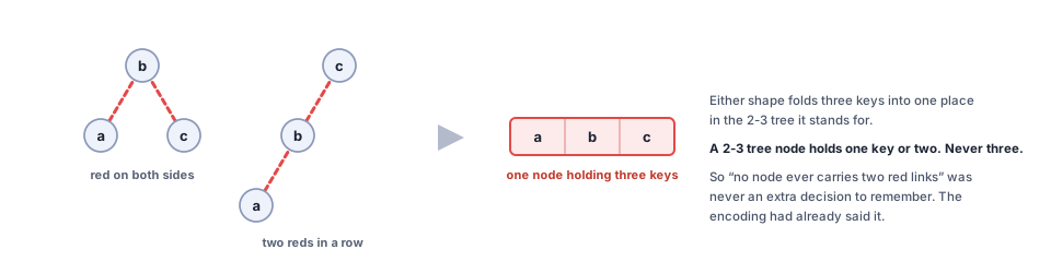
Start with the two red-link rules. They fall straight out of the encoding instead of having to be stated and remembered. Take the rule that no node ever has two red links touching it. Suppose one did: two red links attached to one node, whether both hanging below it or one chained off the other. Either way, that’s three nodes standing in for one local piece of structure: three keys folded into what’s supposed to be a single 2-3 tree node, and such a node holds one key or two, never three. So the rule is part of the encoding itself: it restates, in links, what a 2-3 tree can contain.
The height guarantee comes out of the same encoding, just as directly. Every 2-3 tree has all its leaves at the same depth, by definition, before any coloring enters the picture. Black links are exactly the links between separate 2-3 tree nodes; red links are the internal disguise joining two binary nodes that are secretly one of them. So counting black links from the root down to any leaf is just counting 2-3 tree nodes along that path, and every path has the same count, automatically. No outside check is needed: the equal count follows from what a black link was defined to mean.
The three repair rules tell one connected story. Insert into a 3-node and the new key attaches somewhere in that pair by a red link. For a moment, that spot in the tree is the encoding of a node with three keys, a shape that can’t exist in a 2-3 tree, only in this temporary binary disguise of one. Which rules fire next, and in what order, depends only on where among the three keys the new one landed.
Land as the smallest of the three and the new red link attaches below the pair’s smaller node, on the left, already two left-leaning reds in a row, the shape rotate right resolves by folding the pair into one node with a red link on both sides. Land as the largest and the new red link attaches to the pair’s larger node, on the right, but that node’s left side already carries a red link to the smaller node, so both reds are already on one node, no rotation needed. Land in the middle and the new link attaches between the pair’s two nodes, leaning right where it should lean left. rotate left straightens that inner link into the same two-lefts-in-a-row shape the smallest case starts with, and rotate right finishes it the same way.
However it got there, the outcome is the same: a node with red links on both sides, exactly the shape the no-two-reds rule forbids, exactly what a 2-3 tree does when a 3-node takes a third key: split the node and push the middle key up. That split, replayed as a color change instead of a physical rearrangement, is flip colors: both links turn black, the node stops pretending to hold three keys, and a single red link carries the pushed-up key to the node above, ready to repeat the same story one level higher if it has to.
None of the rules from before were arbitrary. Each one is what happens when you try to keep a 2-3 tree’s shape intact while forcing it to live inside a node that only has room for one key at a time.
2.6.4 Deletion
Deleting a node needs one more trick beyond the three repair rules above. Those rules run on the way back up, fixing the red links an insertion left behind, and they don’t help once a node already has to disappear. Deletion has to arrange things on the way down, before it gets there.
Here is the whole idea in one sentence, before any of the machinery. The walk down maintains an invariant: the node the walk is about to step into is never a bare 2-node. Either the link into it is red, or the link to its left child is. Either way, in the 2-3 picture it is part of a node holding two keys, so it has a key to spare. A node that is neither is holding one key with nothing to spare, and deleting through it would leave a gap in the black count. So Sedgewick’s fix is to make sure the walk never arrives at one: arrange the spare before stepping down, not after.
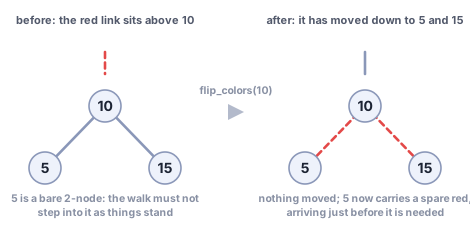
That is the push. Walking down toward the key to delete, push a red link down ahead of the walk whenever the next node would otherwise be bare. The red comes down from the node above; only when the sibling next door has a spare of its own is one borrowed from there instead: move_red_left pushes a spare red link down-and-left before the walk continues left, move_red_right is the mirror image continuing right. By the time the walk reaches the key being deleted, that node is guaranteed to already be carrying a spare, so removing it can never leave a gap behind; the three ordinary repair rules, run again on the way back up, clean up whatever the push disturbed.
Notice that this makes flip_colors serve two purposes. On the way up from an insert it turns a node red and its two children black, sending a red link upward. Run on a node that is already red with two black children, the very same three flips send a red link downward instead, which is exactly the borrowing this walk needs. That is why it’s written to flip all three colors rather than to set them: one repair, used in both directions.
Read move_red_left and move_red_right below as a black box: hand either one a node whose next step is bare, and it hands back one whose next step isn’t. You do not need to hold their bodies in your head to read delete_min, and the line in delete_min that tests is_red(nxt) or is_red(nxt.left) is simply the invariant above, written out.
That is the repair. Here is the walk that uses it, and it can be read knowing only what move_red_left promises, not how it delivers: hand it a node whose next step would be bare, and it hands back one whose next step isn’t.
delete_min is the trick in its simplest form: walk left, pushing a red link ahead of the walk whenever the next node would otherwise be a bare 2-node, until there’s no left child left to descend into. It is worth more than it looks. Deleting the smallest key is a modest operation on its own, but this same walk comes back later as the engine of general deletion, and the name will stop describing what it is for at that point.
That recursion leans on a precondition, one more case of the promise-keeping idea the whole red-black tree runs on: delete_min may only be called on a node that is itself red, or that has a red link on its left. Every recursive step arranges that before descending, which is the entire point of move_red_left. But the first call has nobody above it to arrange anything, so the caller has to do it by hand: color the root red before starting if both of its links are black, and color it back to black when the walk is finished.
What follows is one trace of that walk, step by step. If the invariant above already feels inevitable, skip ahead to the paragraph that begins “Deleting an arbitrary key” and carry on. Nothing later depends on having read the trace. It is here for the reader who wants to watch the machinery move once before trusting it.
Watch it run on the tree those five keys built: 20 at the top, 10 on a red link to its left carrying black 5 and 15, and black 30 on the right. Take out the smallest key, 5.
At 20. Is the walk about to step into a bare 2-node? Its left child 10 arrives on a red link, so no. There is already a spare red link down that way. The walk descends without touching anything.
At 10. Now look one step further ahead, which is the part that matters: the next node is 5, and both 5 and 5’s own left side are black. That is a bare 2-node, precisely what must never be deleted through. So move_red_left fires. flip_colors(10) turns 10 black and turns both its children, 5 and 15, red. Nothing moved; a red link that was sitting above 10 is now sitting above both its children, 5 included, pushed one level down the walk, arriving just before it’s needed. (The sibling check inside move_red_left looks at 15’s left for a spare red grandchild, finds none, and skips its rotation.)
At 5. It has no left child, so the walk returns None and 5 is gone. (Returning nothing is safe rather than lossy: in this tree a node with no left child can have no right child either. A red right child would lean the wrong way. A black one would give the path through it one more black link than the path through the empty left side, which the black-count rule forbids.) And because 5 was carrying a red link when it went, removing it cost the tree no black height anywhere, which is the entire reason for having pushed that link down.
Back up at 10. Its left side is now empty and 15 sits on its right on a red link: a right-leaning red, which the lean-left rule forbids. fix_up rotates left at 10, bringing 15 up into its place and sending 10 down to the left on a red link. At 20, nothing is broken; the root is colored black and the walk is over.
The tree that leaves behind is 20 at the top, black 15 on its left with red 10 beneath it, black 30 on the right. Four keys, every rule intact, every path still crossing the same number of black links: bought with exactly one color flip on the way down and one rotation on the way back up.
Deleting an arbitrary key rather than always the smallest is the same idea, run in both directions at once. Walk toward the target, calling move_red_left or move_red_right depending on which way the walk turns. Once the target node is reached, splice it out exactly the way a plain binary search tree would: copy the successor up if it has two children, remove it directly if it doesn’t. That last step is safe now, and it wasn’t before: the walk down has already guaranteed this node is never a bare 2-node.
Watch it once, on the tree those same five keys built, taking out 20: the key sitting at the very top. You might expect the work to happen up there. It doesn’t.
At the top. The walk compares first: 20 is not smaller than 20, so this is the here-or-right branch, and that branch opens with one rule. If this node has a red link on its left, rotate right. In a left-leaning tree the right side never has a red link of its own, so before the walk might turn right, it brings one over from the left. Node 20 has a red link on its left, so the tree tips. 10 comes up to the top, and 20 slides down to the right, arriving on a red link. Nothing has been deleted yet. The target has simply been moved somewhere safer to work, somewhere it already has the spare that deletion needs.
At 10, now on top. The walk is standing on 10, and 20 is larger, so it turns right. Is the next node bare? No: 20 has just arrived there on a red link, so it already carries a spare, and move_red_right has nothing to do. The walk steps down.
At 20, one level down. This is the key we want, and it has nodes on both sides, and a node with two children cannot simply be spliced out, because one hole cannot hold two subtrees. So it is not removed at all. Its key is replaced by a neighbor in sorted order, and there are exactly two candidates: the predecessor, the largest key on the left, or the successor, the smallest key on the right. Either works, and the two are mirror images. This tree takes the successor: the smallest key on its right, which is 30. But the walk has to be able to step down that side first, and both 30 and 30’s left side are black. move_red_right fires. flip_colors turns 20 black and turns 15 and 30 red, and the right side now carries a spare.
The substitution. Copy 30’s key into this node, then run the delete_min walk on the right side: the same walk as before, on a side that now has what it needs. This is where the earlier walk earns its keep, and where its name becomes misleading. Here the walk is removing the successor from the place it used to live. It can, because the successor is the minimum of the right side: the leftmost node of the right subtree, so it has no left child, which is precisely the easy case. The two-children problem is never met twice. The right side is only the one node, holding a red link when it goes, so removing it costs no black height anywhere. What’s left here is a node holding 30, with 15 hanging red on its left.
Back up. fix_up looks for the three broken shapes and finds none; the top node is already black. Done. Four keys (10 at the top, 5 on its left, 30 on its right with 15 red beneath it), every rule intact.
The thing to take from that is the first step, not the last. The repair that mattered was a rotation that happened before any deleting, whose only job was to put the target somewhere it could be deleted safely. That is what “arrange it on the way down” means in practice.
It is also where the match with the 2-3 tree stops. The walk down borrows ahead of time, the way the B-tree’s deletion tops up a node before stepping into it, and on the way it passes through shapes no 2-3 tree has: a red link on each side of a node, a red link leaning right. The tree it leaves is always valid, so it always reads as some 2-3 tree, but not always the one a 2-3 tree’s own deletion would give. Build the 2-3 tree of 24 and 35 over 9, 31 and 38-39, and take out 31. The 2-3 tree borrows from its neighbor: 38 rises, 35 comes down, and the result is 24 and 38 over 9, 35 and 39. The left-leaning tree merges instead and ends as 35 over 9-24 and 38-39. Same keys, same height, both valid, different trees.
One detail in there is worth stopping on, because it contradicts something settled earlier in this chapter. The plain tree’s deletion section came down on the side of moving the node rather than copying the key out of it, so that outside code still holding that node isn’t left pointing at nothing. This tree copies the key on purpose. The trade comes out the other way here, because a node holds something a plain tree’s node didn’t. It holds a color, and that color is a claim about the path it sits on. Copy a key and every color stays exactly where it was and every claim still holds. Move a node and its color travels with it into a place whose black counts were already settled, and both ends need repairing. The guarantee you bought earlier is real; here it costs more than it is worth, and this structure declines to buy it.
Key idea: a bound on height is not a bound on rotations
Both red-black trees keep the height, and so the work of every operation, proportional to \(\lg n\). Only the standard tree also bounds the structural change: \(O(1)\) rotations, at most two per insert and three per delete [5]. The left-leaning tree runs fix_up at every node on the way back up and can rotate at every level, so its bound is \(O(\lg n)\) rotations per operation, not \(O(1)\). On trees of 4,096 random keys it took up to 11 rotations for one insert and up to 15 for one delete, about 5 per delete on average (computed 2026-09-29 by scripts/rotation_counts.py). Where each rotation has a cost of its own, that is the reason to choose the standard tree.
2.6.5 What a proof checks, and what it doesn’t
The two trees so far run on invariants: promises true again after every operation, so later steps can lean on them instead of rechecking. The plain tree’s ordering rule is kept by every insert, and lookup simply trusts it and walks; the red-black tree’s rules may break for a moment during an insert, and the repairs on the way back up restore them before the insert counts as done.
Tests hold every piece of code printed in this chapter to the companion library on every change; the contracts chapter, under “How this book checks itself”, sets out what that does and doesn’t guarantee. For the red-black tree the library goes one step further, to a proof, and a proof starts from a definition. Here is a valid left-leaning red-black tree as the proof assistant, Lean, defines it, in the companion library at lean/AlgoDesign/Searching/LLRB/Spec.lean:
def Valid (t : LLRB α) : Prop :=
  Sorted t ∧ RootBlack t ∧ LeftLeaning t ∧ NoRedRed t ∧ BlackHeightOk t
Read it as the chapter’s five rules joined by “and”, because that is all it is: the keys are in order, the top of the tree is black, red links lean left, no two red links touch, and every downward path crosses the same number of black links. The notation is plain: ∧ is “and”, α stands for whatever type the keys have, and Prop means “this is a claim, which may be true or false of a given tree”.
What that buys is narrower than it sounds, and the honest version is worth more than the impressive one. A machine has checked that inserting into a tree satisfying those five leaves a tree still satisfying them, and the same holds for deletion: the arbitrary-key walk this section spent its longest stretch on preserves all five, and removes exactly the key you asked for and no other. The deletion proof took considerably longer than the insertion proof, for a reason the walk itself makes plain: it rearranges the tree on the way down, so the node it recurses into is often no longer the one it was looking at. It has not checked the Python printed above; that is held to the same behavior by tests, not by proof. And it says nothing about whether those five are the right five. That judgment is still a person’s, which is why the chapter spent its time on where each rule came from rather than on the fact that a machine agrees.
There is a sharper way to see the limit, and it happened to this book’s own library. An early version of the deletion definition spliced out a node on reaching an empty right child, which reads correctly and is one clause short of correct: it has to reach an empty right child and be standing on the key being deleted. Without that second condition, whenever the key you asked for wasn’t there at all, it quietly removed the largest key below it instead. The definition type-checked: Lean accepted it as well formed. It was proved total: it always terminates. Every proof already written about it still went through, because none of them said anything about which key comes out. What caught it was a property test comparing it against a plain list over thousands of random sequences.
That is the shape of the guarantee: a proof assistant checks the properties you thought to state, with complete rigor, and is silent on the ones you didn’t. Deciding what to state is the part that is still yours.
Back to the tree itself. It can no longer lean into one long line the way it did before, so the height guarantee holds. But every one of these operations, comparing, rotating, flipping, still means chasing one pointer at a time, node to node, down a single path. That assumption, that reaching a key means walking to it one node at a time, is about to break.
2.7 Frankenstein
B-tree
2.7.1 Blocks and fan-out
Everything so far has quietly assumed that looking at any key costs about the same as looking at any other. Call that the RAM model, the same assumption named in the contracts chapter, under “The memory hierarchy”.
Real memory doesn’t hand you one key at a time for free. It hands you whole chunks, whether you asked for a chunk or not: a disk sector, a page, a block. Fetching that block is the expensive step; once it has arrived, looking through everything sitting inside it is comparatively free. Call this the I/O model, and call the expensive step itself a block transfer: the cost that matters here is how many separate blocks you had to fetch, however many keys you then compare inside them.
If fetching a block is the expensive step, and everything already inside it is nearly free to look through once it’s arrived, what would you change about a node to make each expensive fetch worth more? Before reading on, decide what a node should hold instead of a single key.
Two minutes. One sentence is a complete answer.
A tree built one key per node wastes that free look inside each block. Walking node to node down a single path, comparing one key at a time, pays for a full block transfer at every node, even though each block probably had room for dozens of keys riding along for free. Almost all of what got fetched goes unused.
So change what a node is willing to hold. A single node in this tree can hold several keys at once, not just one. That’s the whole idea: one expensive block transfer now buys many cheap comparisons inside the node you just fetched, instead of paying for a fresh block transfer on every pointer hop. This is a B-tree.
You already know this idea, though probably not about keys. You don’t walk to the kitchen five times to bring back five things. You go once and carry an armful, because the walk is what costs and what’s in your arms is nearly free. Anyone who has ever been halfway up the stairs and thought “while I’m going anyway, I’ll take the rest” has had this thought, and that thought is all there is to the B-tree.
That’s the trade a B-tree makes, in one sentence: a node holding one key means a separate trip for every key, so make the node hold an armful. The rest of the tree stays as it was. It still branches, it still compares, it still walks down one path. It just refuses to make the trip for one thing.
Here is where the kitchen stops being the right picture, and the difference is the part that matters. Going to the kitchen, you choose what to carry back. Storage doesn’t work that way. You ask for one thing and it hands you that thing together with whatever happens to be lying next to it, because a block is a block whether you wanted all of it or not. You don’t get to fill your arms; your arms get filled for you. That turns what looked like a free choice into a design obligation. The neighbors are coming along regardless. So the armful is worth carrying only if the things sitting next to each other are things you would have wanted next to each other anyway. That is precisely why the keys inside a node are kept in sorted order rather than thrown in as they arrive: sortedness is what makes an unchosen armful useful.
Look at what that makes each node: a short sorted array, the sorted row from the start of this chapter, fast to search once it has arrived. And the nodes hang off one another the way single keys did in the search tree, so the whole thing can grow without anything being shoved along a row. The B-tree is stitched together from two earlier designs, the array’s cheap scanning inside each node and the tree’s cheap growth between them, each covering the other’s weakness. A creature sewn from parts that were never meant to share one body, and it walks.
Put numbers on it. Give every node room for a thousand keys, and to be pessimistic, let those nodes sit only half full, which is the least a B-tree ever allows:
| Keys stored | Trips, with a thousand keys per node | Trips, one key per node |
|---|---|---|
| 500,000 | 3 | 19 |
| 50,000,000 | 3 | 26 |
| 62,500,000,000 | 4 | 36 |
Fifty million keys, three trips. The right-hand column is what the same collection costs a tree that insists on one key per node: twenty-six separate journeys to twenty-six separate places. Both columns are logarithms (the fixed-fraction rule from the sorted row, still running), but one takes its logarithm in a base of about 500 (a thousand slots, kept half full) and the other in base 2, and on real hardware every step in that right-hand column is a fresh expensive fetch. The gap between the two columns is the reason the B-tree exists.
2.7.2 Search, insertion and node splitting
Here’s what that looks like on actual keys. Give each node room for up to three keys and up to four children, small enough to trace by hand, big enough to show a split. Build one up by inserting 10, 20, 5, 6, 12, 30, and 7, in that order. All but one slide into whichever node they land on. The exception is 6: by then the root holds 5, 10 and 20 and is full, so it splits first, the move you will watch in detail with 17 below. After all seven, the tree has settled into two levels: a root node holding a single key, 10, with two nodes hanging off it: a left node holding 5, 6, 7, and a right node holding 12, 20, 30.
Now search that tree for 20. Start at the root and scan its one key: 20 is bigger than 10, so there’s nothing more to check here. Descend into the gap to the right of 10, which is the right node. That’s the second block transfer. Fetch it, and scan the three keys sitting inside: 12, then 20, a match. Two nodes fetched, three keys compared in all, one at the root and two below it, and the key is found. With seven keys the saving is small: a balanced tree of single keys reaches any of them in at most three nodes, this one in at most two. The table above is what that gap becomes as the keys grow.
Insertion is where the interesting part happens. Insert 17. Walk down the same way a search would: at the root, 17 is bigger than 10, so head for the right node. But the right node is already holding three keys (12, 20, 30) and three is all it’s allowed to hold. There’s no room to just slide 17 in. So split it first, before descending any further.
Splitting means: take the middle key of the full node (that’s 20) and push it up into the parent, the root. The two keys on either side of it, 12 and 30, stay behind, but now in two separate nodes instead of one: a node holding just 12, and a node holding just 30. The root, which used to hold only 10, now holds 10 and 20, with three nodes hanging off it instead of two. Only after the split is finished does 17 actually get placed. It belongs in the gap between 10 and 20, which is the node holding 12, so it slides in next to it: 12, 17.
The end state: a root holding 10, 20; a left node holding 5, 6, 7; a middle node holding 12, 17; a right node holding 30. One full node that had no room left turned into two nodes with room to spare, and the tree grew a little wider at the top instead of a little taller down one path. That is the split the red-black tree’s third repair made: the middle key goes up, and the outer two stay behind as nodes of their own, here paid in whole blocks of keys instead of single ones.
Notice which direction the key traveled, because it is the reason this tree can promise what it promises. A split sends its middle key up, never down. Pushing down would lengthen one path and leave the others alone, and the moment two leaves sit at different depths the whole cost argument collapses: a lookup would no longer cost the same wherever it landed. Pushing up lengthens every path at once or none of them: the only way this tree ever gets taller is for a split to reach the root and have nowhere left to push, at which point a brand-new root appears above the old one and every leaf gets one step deeper together. That is what keeps all the leaves level, and it is why a B-tree grows at the top rather than at the bottom. The plain search tree grows at its leaves; the 2-3 tree behind the red-black one grows the B-tree’s way, by a new root when a split reaches the top.
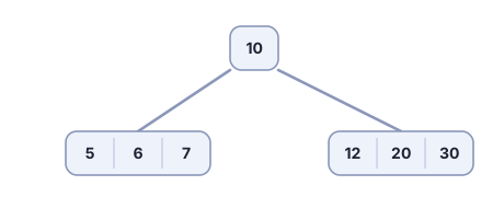
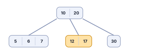
Here’s the same idea, interactive. As in the other two widgets, one press is one move: the walk down, the full node it meets, the split, and then the key going in, each shown separately. Watch the order in particular: the split always happens before the arriving key gets anywhere near the node.
That’s enough to see the shape of it. The code below gives the exact mechanics of a split, and after it the section picks up how tall that makes the tree, how full these nodes really stay, what a B*-tree does to improve on that, and how deletion runs the whole splitting story in reverse.
One letter in that code needs its meaning before you read it, and gets its proper treatment a few pages on. self.t is how wide a node is allowed to be: a node holds at most \(2t-1\) keys, so the tree you just traced, with three keys to a node, had \(t = 2\). That is all you need here.
This structure is also the thing promised back at the start of this chapter. The B-tree [14] is what sits under the indexes of most databases you’ve ever queried (often in a variant called a B+-tree, which keeps all the actual data in the leaves), and under the directories of nearly every filesystem you’ve ever saved a file to: the design in this chapter doing the most quiet work in the most places.
2.7.3 B-tree height
So far the argument for the B-tree has been in words only: fat nodes mean fewer trips. Now put one number on it, because the number is the reason anybody bothers.
Call \(t\) the minimum degree: the number chosen so that one node fills one block. The root is allowed to be thin, with as few as two children. Every node below it holds at least \(t-1\) keys and has at least \(t\) children. In the small tree you just traced, \(t\) was 2, which is why its nodes held up to three keys and had up to four children.
One word before it costs you something, the same deal as node earlier. Most sources, and most exam papers, do not say minimum degree at all. They say a B-tree of order \(m\), where \(m\) counts the most children a node may have. The tree you just traced is order 4. The two are the same structure counted from opposite ends, \(m = 2t\), and the literature is genuinely inconsistent about which one “order” means, so check before you trust it. This book counts with \(t\) because \(t\) is what shows up in the arithmetic.
So going down one level multiplies the number of nodes by at least \(t\), and in a tree holding \(n\) keys no leaf sits more than \(\log_t \frac{n+1}{2}\) steps below the root. Now notice what \(t\) does there. Since \(\log_t n = \lg n / \lg t\), every doubling of \(t\) knocks another slice off the height. Making a node fatter divides the whole walk down, instead of shaving a constant off it.
Put a real block under it. A 16 KB page, 16-byte keys and 8-byte child pointers, leaves room for roughly 680 keys per node, so \(t\) is about 340. A trillion keys is then \(\log_{340}(10^{12}/2) \approx 4.6\), so at most four steps below the root: five levels, five block fetches, worst case, ever. Hold the first two levels in memory, which is what happens anyway once a database keeps the pages it touches most, and a lookup anywhere in a trillion keys costs about three trips to disk.
Run the same trillion keys through the red-black tree. No binary tree can be shorter than \(\lg 10^{12} \approx 40\) levels, and the red-black tree’s looser rule allows up to about twice that, so call it forty at the very best and eighty at worst. Put that tree on the same disk and every one of those hops is its own block fetch, because a pointer can land anywhere. Five against forty, from one change: let a node hold an armful.
That is the whole case for the B-tree, and notice what kind of case it is. Both trees are \(O(\log n)\). The complexity class is identical; what differs is the base of the logarithm, and the base is set by how much one trip brings back.
All that extra scanning inside a node only pays for itself because of where the real cost lives. Doing more cheap work inside a node to avoid an expensive trip to the next one is worth it exactly when reaching a node costs vastly more than comparing keys already in your hand: \(C_{\text{access}} \gg C_{\text{compare}}\). Wherever that gap is wide enough, a few wide nodes beat many narrow ones, every time.
The worst-case picture undersells how full these nodes actually stay in practice, and the real number is prettier than the guarantee. A node is only required to hold half its capacity; left to fill under random arrivals, the average settles at \(\ln 2 \approx 69\%\) full [15]. Roughly a third of the space sits empty, on average: the standing price of never having to reorganize everything at once.
A B*-tree buys some of that space back. Instead of splitting a full node the moment it overflows, first try to shift a few of its keys sideways into a neighboring node that still has room, and split only when the neighbors are full too, and when that finally happens, split two full nodes into three roughly two-thirds-full ones rather than two half-full ones. That single change lifts the average occupancy from 69% to about \(2\ln(3/2) \approx 81\%\) [16]. Fuller nodes, fewer of them, paid for by checking a neighbor before every split.
2.7.4 Top-down insert and delete
Searching still starts at the root and still walks downward, but each stop now does more work before moving on. Scan across the keys sitting on that node (or, once there are enough of them, binary-search across them the way you did with the sorted row) to find which gap between two keys the one you’re after falls into, then step down into whichever node hangs off that gap. Adding a key follows that same walk to the node where it belongs and slides it in alongside its neighbors. Any full node met on the way down is split before the walk enters it, its middle key pushed up into the node above, which the walk has already made sure has room, so a split never has to travel back up.
Deleting a key runs the same discipline in the same direction: down, once, and never back up. Insertion refuses to step into a node that is already full. Deletion refuses to step into one that is already at the minimum, because taking a key out of such a node would leave it underflowing, holding fewer than the \(t - 1\) keys every node but the root must keep: the floor of the same rule whose ceiling made splitting necessary in the first place. So top it up first, before descending any further.
Topping up tries the cheap option first: redistribute a spare key over from a neighboring node that has more than the minimum, the neighbor’s nearest key moves up into the parent, and the parent’s key that separated the two moves down into the thin node, so the ordering still holds. Only when neither neighbor has a key to spare does it fall back to merging: fuse the node with a neighbor and pull the separating key out of the parent to hold them together. The order is fixed, and it decides which keys end up where: borrow from the left neighbor if it can spare one, otherwise from the right, and only then merge, with the left neighbor when there is one. Either way the node you are about to step into now has room to lose a key, so nothing underflows and nothing has to be repaired on the way back up. Every node on the path is fetched once and written at most once, and no ancestor has to be held in reserve against a repair that might come climbing back [5].
Merging is the move that can shorten the tree, because pulling a key down out of a parent is what empties the parent. If the parent is the root and that key was its last, the root is discarded and its one remaining child becomes the new root: the only way this tree ever loses a level, the exact mirror of a root split being the only way it ever gains one.
Doing the repair on the way down rather than on the way back up is visible from the outside, and worth knowing before you read the code. A node gets topped up because it sits at the minimum, not because the deletion turned out to need it, so a tree can lose a level on a deletion that would never have underflowed anything at all. That is the price of never climbing back. Other presentations take the opposite trade: delete first, then repair upward if a node turns out to have underflowed, doing less work on a deletion that disturbs nothing and paying for it with the climb [12], [17].
Watch both of those on the tree you just built, the one the split left behind: 10 and 20 on top, with 5-6-7, 12-17 and 30 hanging under it.
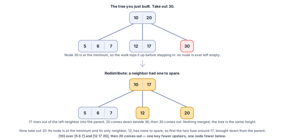
Take out 30. Its node is holding the minimum already, so it gets topped up before anything is taken out of it. The cheap fix is available: the neighbor to its left, 12-17, has two keys and can spare one. But 17 doesn’t move sideways into the thin node: it goes up. It rises into the parent, and 20, which had been sitting there separating the two, comes down into 30’s node, which now holds 20 and 30. Only then is 30 taken out, leaving 20 behind. The ordering still reads correctly left to right, and nothing merged, so the tree is exactly as tall as it was.
Now take out 20, which is sitting where 30 used to be. Its node is at the minimum again, and this time the cheap fix isn’t available: its only neighbor holds 12 and nothing more. So the two fuse instead, and the key that had been separating them, 17, comes down out of the parent to join them into one node holding 12, 17 and 20. Then 20 is taken out, leaving 12 and 17. The parent is left holding just 10, with two children instead of three.
That last move is the one that can shorten the tree. Pulling a key down out of a parent is exactly what thins the parent out, and because the walk tops up every node it is about to step into, a parent that has been thinned is topped up in its turn on the way down. Take enough out and the root is left holding nothing, at which point it is thrown away and its one remaining child becomes the new root: the tree loses a level, in the only way it ever does.
Last, take out 10, which sits in the root itself rather than in a leaf. A key in an internal node cannot just be removed: it is the separator holding its two children apart, and without it the node would have one child too many. So it is replaced, the same way the red-black tree replaced 20: by a neighbor in sorted order, fetched from the bottom of the tree, where removing a key is easy. The predecessor, the largest key to its left, is 7, and the left child 5-6-7 can spare a key, so 7 moves up into the root. What is left is 7 on top, with 5-6 and 12-17 below. Had the left child been at the minimum, the successor from the right child would have come up instead, 12 here. Had both children been at the minimum, neither could give anything up, so the two merge, with the key being deleted pulled down into the middle of the merged node, and the walk carries on inside it, where the key is now an ordinary one to take out. In a taller tree the predecessor sits at the bottom of the left subtree’s right edge, and the walk down to it tops up every node before stepping into it, exactly as before. The red-black tree reached for the successor; this code tries the predecessor first. Either is correct, provided it comes from a side that can afford to lose a key.
2.7.5 The B-tree, question by question
The contracts chapter listed seven questions that making a design runs through. Here they are, answered once, for the B-tree, with this chapter’s own numbers. The same seven, answered for a workload nobody has named yet, are how a design that does not exist yet gets made.
| question | the B-tree’s answer |
|---|---|
| What is the workload, and what does it ask for most often? | An ordered collection far larger than memory: lookups, range scans and updates, each one a walk to one key. |
| Which resource is scarce, and so what are you paying for? | Block transfers. Comparing keys inside a block already fetched is nearly free; fetching the next block is not. |
| What can no design beat? | A fetched block of \(B\) sorted keys can end a comparison in at most \(2B+1\) ways: equal to one of its keys, or in one of the \(B+1\) gaps around them. Telling apart \(n+1\) answers, one per key and one for “not here”, takes at least \(\log_{2B+1}(n+1)\) fetches: the decision tree again, with \(b = 2B+1\). |
| Which promise will you keep, stated on the meaning? | The tree holds exactly the keys inserted and not since deleted, and every query answers about that set. The rules that keep it cheap: every node but the root holds between \(t-1\) and \(2t-1\) keys, in order, and every leaf sits at the same depth. |
| Which idea keeps that promise cheap? | Work in blocks, so one fetch buys a whole node; slack in the levels below, so an arrival never shoves; grow at the root, so every leaf stays level. |
| What does it cost, and what does it refuse to cover? | \(\Theta(\log_t n)\) fetches per operation, within a constant factor of the floor because \(t\) is about \(B/2\): five fetches for a trillion keys at \(t \approx 340\). Nodes sit about 69% full on average and may sit half empty. It refuses to make a write cheaper than a trip to the one leaf its key lives in. |
| What change would make you reconsider? | Writes arriving faster than reads, so that the trip to the leaf becomes the cost that matters. That is the LSM-tree’s workload. |
2.7.6 ★ Cache-oblivious variant advanced
Cache-oblivious layout (van Emde Boas)
A careful reader has a question by now. The B-tree fits its node to the block, but the memory hierarchy in the contracts chapter has several levels, and each moves data in blocks of a different size: a cache line of a few dozen bytes, a page of a few kilobytes, a flash block much larger. A node sized for one of them is the wrong size for the others. Which one is it supposed to fit?
Surprisingly, you do not have to choose. Take a plain binary tree and lay it out in memory by one recursive rule: cut the tree at half its height, store the top half first, laid out by the same rule, then each subtree hanging below the cut, one after another, each laid out by the same rule. Whatever the block size turns out to be, at some depth of that recursion the pieces are about the size of a block, and each is stored contiguously. So a search reads within a small constant factor of the blocks a tree tuned to that size would, without the layout ever having known the size. This is the van Emde Boas layout, and a structure that gets its block-transfer bound this way, with no block size anywhere in its code, is called cache-oblivious [18].
What that buys is easiest to see measured. A tree of about a million keys, laid out five ways; each search charged one transfer per distinct block it touches, averaged over 2,000 random searches (computed 2026-09-29 by scripts/cache_oblivious_table.py, block sizes counted in nodes):
| layout | blocks of 16 | blocks of 256 | blocks of 4,096 |
|---|---|---|---|
| level by level, no tuning | 16.9 | 13.0 | 9.0 |
| tuned to 16 | 5.0 | 4.1 | 3.1 |
| tuned to 256 | 10.9 | 3.0 | 2.9 |
| tuned to 4,096 | 13.9 | 6.0 | 2.0 |
| van Emde Boas | 7.6 | 3.8 | 2.1 |
Each tuned layout wins at the size it was tuned for, and the one tuned for big blocks is almost as bad as no tuning at all when the blocks turn out small. The recursive layout never wins a column and is never far behind the winner in any of them. That is the trade, and it is the right way to read the idea: the appeal is portability. A structure tuned to the one level that actually dominates a given machine can do as well there, and a standard book on database internals describes the cache-oblivious B-tree while noting no implementation of it outside research [17]. Reach for it when the code has to run well on machines you will never see.
That completes the first chain of fixes. Every fix along it, ring to tree to red-black tree to B-tree, took the workload as fixed and changed the structure to survive it. What if the next thing to break isn’t the structure at all: what if it’s the workload?
2.8 I’ll pay it back later
Log-structured merge-tree (LSM-tree)
The B-tree fixed fetching. One trip brings back an armful, so finding anything costs three journeys instead of twenty-six. All of that stays for what happens next. What changes is what the day looks like.
Until now, things have mostly been looked up. Now they mostly arrive. Something new turns up every few seconds, all day, and each one has to end up where it belongs so it can be found later.
Follow one arrival. Walk to the place it goes. Put it away. Walk back. The next thing to arrive has nothing to do with the last one (things show up in the order the world sends them, not in the order they’re stored), so that’s a walk to somewhere else entirely. And every so often the place you’re putting things is full, so you have to rearrange it, and its neighbors, before the new thing fits.
The tree is keeping every promise it made. But look at what the day is actually being spent on: mostly walking to the place where putting away happens. A short trip is wonderful when somebody is standing there waiting for an answer. It is pure overhead when nobody is waiting for anything at all, and the only thing that has to end up true is that the item is stored.
There is something else hiding in that trip, and everything that follows turns on it. The walk was never logically necessary. A search has to go find the thing. That is the entire question being asked. But storing something doesn’t need to know where the old version sat. It only needs the collection to end up knowing a newer one exists. Every design so far has quietly assumed otherwise: that changing something means finding it first, and changing it in place.
Suppose you were forbidden to make the trip at the moment something arrives. Things still have to end up findable, and you must still be able to answer “where is the X?” But an arrival itself may only be written down, right where you’re standing, without going anywhere.
Before reading on, design that. Where does an arriving thing go, how does the proper place ever get updated, and, the part that costs you later, how does a lookup work afterwards, when the answer might be in what you wrote down or in the place it eventually went?
Ten minutes, and write the lookup rule as an actual sequence of steps rather than a description. You’re done when your rule gives a definite answer for a thing you wrote down twice.
2.8.1 Writing
So stop writing in place. Keep new writes in a small, sorted buffer held entirely in memory, a memtable, and once it fills up, don’t merge it into anything: write it straight to disk, whole, sorted, and untouched from then on. That is a flush, and the file it makes, an SSTable (sorted string table), never gets modified again, finished, permanent. A key updated later doesn’t go back and change the old file; it just gets written again, into whatever memtable is currently open, with a newer timestamp riding along. This is a log-structured merge tree, LSM-tree for short [19]. The two words in its name are the whole idea. Logged: writes only ever get appended, one after another, never written into the middle. Merge: the accumulating pile of files gets merged back down later, off the hot path: the short sequence of work a single write has to wait for before it can be called done.
That shape is worth fixing in your head before any of the mechanism arrives, because it is what an LSM-tree looks like, the way a red left-leaning link is what the red-black tree looks like and a fat node is what the B-tree looks like.
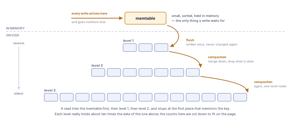
Everything in the rest of this section is a detail of that picture: what “written once” buys, what a lookup has to do now that an answer might be on any level, and what the merging downward costs.
Here is that idea at a scale you can hold in your head, and it is the chapter’s opening question turned around: instead of losing your keys, keep a note of where everything went. Write arrivals on a list, and once the list has three things on it, make one trip and put all three away properly. Six things happen.
| What happens | The list afterwards |
|---|---|
| charger goes in the desk drawer | charger: desk drawer |
| passport goes on the top shelf | charger: desk drawer, passport: top shelf |
| scissors go in the kitchen drawer | charger: desk drawer, passport: top shelf, scissors: kitchen drawer, full |
| (one trip: the list is sorted and filed away as a sealed page) | list empty; Page 1 = charger: desk drawer, passport: top shelf, scissors: kitchen drawer |
| charger moves to the bedside table | charger: bedside table |
| scissors are thrown out | charger: bedside table, scissors: gone |
| umbrella goes on the hallway hook | charger: bedside table, scissors: gone, umbrella: hallway hook, full |
| (one trip) | list empty; Page 2 = charger: bedside table, scissors: gone, umbrella: hallway hook |
Two things in that table are the whole trick, and both look wrong at first. Page 1 still says the charger is in the desk drawer. Nobody went back to correct it, and nobody ever will. And the scissors, which were thrown out, are not erased anywhere: Page 2 simply records that they’re gone. Page 1 is sealed. That is the entire point of sealing it: never walk back.
2.8.2 Reading
So the truth about anything is whatever the newest record of it says: the list first, then the pages, newest first. Ask four questions and watch how that works out:
| Question | Where you look | Answer |
|---|---|---|
| Where’s the charger? | list (nothing), Page 2 → found | bedside table, though Page 1’s desk drawer is never consulted |
| Where are the scissors? | list (nothing), Page 2 → found, marked gone | nowhere, because the search stops there and never sees the kitchen drawer |
| Where’s the passport? | list, Page 2 (nothing), Page 1 → found | top shelf |
| Where’s the bicycle pump? | list, Page 2, Page 1: nothing, anywhere | nowhere |
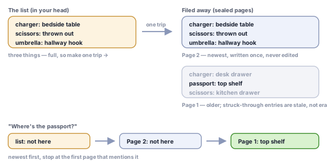
Reading goes newest first and stops at the first page that mentions the thing, which is why an out-of-date entry on an older page does no harm: nothing ever reaches it. Look hard at the last row, though. The bicycle pump was never written down at all, and establishing that took reading every page there is. A question with no answer is the expensive one here, and it gets more expensive with every page that accumulates. Remember that; it comes back shortly.
Writes got cheap, and reading pays for it, differently depending on what’s being asked. Looking up one key is the walk the table above just did: check the memtable, then each file from newest to oldest, and stop at the first one that mentions the key, because by construction that one holds the current truth. Asking for a range of keys can’t stop early, every file might hold part of the answer, so it opens all of them at once and runs a multiway merge across them: one cursor in each file, and again and again, take the smallest key under any cursor and move that cursor on, emitting keys in order and keeping only the newest version of each. One key: stop at the first hit. Many keys in order: reconcile everything.
Each SSTable splits what it holds into two pieces: a data file, the key-value pairs written once in sorted order, and an index locating where each key’s neighborhood begins in that file. Because the data file is already sorted, the index doesn’t have to name every key. It can be sparse, recording only the first key of each block, and a lookup binary-searches that small list to find which block would contain the key, then reads and scans exactly that one block. Sparse is what makes the index small enough to keep in memory; sorted is what makes it able to answer for keys it has never seen, which is what both an absent key and the start of a range scan need. An index that only knew the keys actually present (a hash table, say) could answer point lookups but could not tell you where to begin, and the whole ordered half of this structure’s job would be gone.
2.8.3 Deletion
Deleting can’t erase a byte from a file that’s permanent by design, so a delete writes a tombstone, a record meaning “every older version of this key is dead.” A tombstone is data like any other, and a read has to honor it exactly the way it honors a value. That is why “where are the scissors?” answered nowhere rather than the kitchen drawer. The search met the tombstone first and stopped, which is all it ever does.
2.8.4 Bloom filters
That leaves the expensive case the trace ended on: the key that isn’t anywhere. A lookup for an absent key has no first hit to stop at, so it touches every file before it can say “nobody,” and that is the cost that grows as the pile grows. The standard fix is to put a Bloom filter in front of each file: a small bitmap, cheap enough to keep in memory, that answers “is this key definitely not here?” with certainty and “might it be here?” with a small false-positive rate. A lookup consults the filters first and skips almost every file without reading a byte of it. Nothing about the LSM idea requires Bloom filters, but every major engine ships them, because without them reads for absent keys degrade exactly as fast as writes get cheap. What the engines actually argue about is where to spend the memory: RocksDB will skip building filters on the bottom-most level, which holds most of the data, when the workload is mostly hits rather than misses; Cassandra exposes the false-positive rate per table; HBase shipped with them off by default until 0.96. “Always on, everywhere” is the thing to avoid believing. The filter is a tunable answer to a specific cost.
Skipping a file is safe only because of one property of the filter: it never says “not here” about a key the file actually holds. The read rule depends on that. It stops at the first record it finds, newest first, so every file it skips has to truly lack the key.
Now imagine a filter that could make the opposite mistake. You ask for the charger. Page 2’s filter wrongly says “not here”, so the lookup skips Page 2 and reads Page 1, which still says desk drawer. You get the old answer, and no error. The scissors fare worse: skip the page holding their tombstone, and the lookup finds the kitchen drawer, as if they had never been thrown out.
So the two possible mistakes are not equal. Saying “maybe” about a missing key costs one wasted read. Saying “not here” about a key that is there returns a wrong answer, and nothing afterwards can tell.
The tuning has a derivable answer, and it is not “the same everywhere.” The levels near the top are small, so a few extra bits per key there cost little memory and cut false positives sharply; the bottom level holds most of the keys, so every bit per key there is expensive. The optimum gives the small levels more bits per key than the large one [20]. The question after that is whether to keep re-tuning as the popular keys shift, and a recent analysis finds that the workload enters the optimum only through a logarithm, so a coarse estimate of it loses little [21]. The filter itself has also moved on since Bloom: a cuckoo filter can delete a key [22], a binary fuse filter is smaller and faster for a set that has stopped changing [23], a ribbon filter lets you trade building time for space [24], and an InfiniFilter keeps working when nobody knew in advance how many keys would come [25]. None of them is free of false positives, and none ever will be. A filter smaller than the keys it summarizes has to say “maybe” about some keys it never saw, and how small it can get for a given false-positive rate is a proved lower bound, recently sharpened [26]. The space forces the flaw on every design.
2.8.5 Compaction
Left alone that pile only grows, and every read gets slower as it grows. Compaction keeps it bounded: periodically merge several files into fewer, dropping shadowed versions and spent tombstones along the way. This is where Page 1’s stale claim about the charger finally dies, long after the charger moved: whenever compaction next rewrites those two pages into one and simply declines to copy the older entry forward. Tombstones are what let it do that safely: the scissors’ tombstone is the proof that the kitchen-drawer entry beneath it is dead, and only once both pages are being rewritten together can the tombstone itself be dropped as well.
Leveled compaction, the scheme RocksDB uses, organizes the pile as numbered levels. Each level holds many files of roughly the same size, cut into disjoint key ranges, and each level is allowed to hold about ten times as much total data as the one above it. The top level is the exception, and it is the one that bites: fresh flushes land there whole, so its files overlap each other and a read has to consult every one of them. Letting that level pile up is the classic way an LSM system stalls. When a level exceeds its budget, one of its files is merged into the overlapping files of the level below. Data migrates downward through the levels instead of settling into a few enormous files, getting rewritten each time it descends, which is precisely why this scheme keeps reads cheap (few files to check per level) at the cost of writing the same data several times over on its way down.
The original formulation of this idea used just two components, one in memory and one on disk, merged against each other continuously [19]. Systems in use today use many components instead, arranged in levels or tiers, because merging one enormous disk-resident structure against a small memory one, over and over, rewrites far too much of it per write.
2.8.6 Costs
Everything in the LSM-tree so far has a name in the literature, and the names are worth having because they turn a pile of tricks into one measurable trade. A read that has to consult several files to answer one question is paying read amplification. Data rewritten on every descent through the levels is paying write amplification. Stale entries and spent tombstones occupying space until compaction gets to them are paying space amplification. The three pull against each other: compact more aggressively and read amplification falls while write amplification climbs; compact less and space and read costs grow instead.
Every index faces that tension, the B-tree included, and it has a name, the RUM conjecture (read, update, memory):
Key idea: the RUM conjecture
An index pays overheads on Reads, on Updates and in Memory. It can make any two of them small only by letting the third grow [27]. The B-tree keeps reads and memory down and pays on updates; the LSM-tree makes updates cheap and pays on reads, buying some of that back with memory spent on filters.
Every structure in this chapter sits somewhere on that triangle. A B-tree takes the read-optimized corner: a write goes straight to the one place it belongs, so reads touch exactly one path, and the price is that every write must eventually be applied in the one place its key belongs, which the writer does not get to choose. Real systems soften that by dirtying the page in memory and letting a background pass file many changes at once, but the obligation does not go away, and a whole page gets rewritten for a change of a few bytes. An LSM-tree takes the opposite corner: writes never seek, and the price is a read that may have to ask several files the same question and reconcile the different answers it gets back. Neither is the better structure. They are answers to different questions about which cost the workload can afford.
The LSM-tree is the structure sitting underneath RocksDB, Cassandra, LevelDB, HBase, and BigTable: every one of them a variation on memtable, SSTable, and compaction, tuned differently for whichever corner of that RUM triangle its workload needs most.
2.8.7 Write-ahead log
One more piece keeps the scheme honest, and the list itself shows where the hole is. A list you keep in your head is a wonderful thing right up until somebody interrupts you. Then it’s gone, and the things on it were never put away. You have neither the note nor the filing. Everything written down but not yet filed lives in exactly that gap.
Memory is that list, and it does not survive losing power. A flush is the only moment anything becomes durable, so between flushes there could be a whole memtable of accepted writes with nothing on disk to show for them. So before a write is allowed into the memtable it’s first appended to a write-ahead log: a file that is only ever written at the end, never in the middle, which is about as cheap as writing gets. The log is the difference between holding the list in your head and scribbling it on paper as you go: the scribble is not organized, is not where anything belongs, and is not meant to be read in the ordinary way. It exists so that an interruption costs you nothing. After a crash, replaying the log rebuilds the memtable exactly as it was. And a log segment can be discarded the moment its memtable is flushed, not before: once the page is filed, the scribbles that produced it are redundant. Cheap is not free, though: durability means waiting for the device to confirm the write actually landed, and that wait does not care how sequential you were. It is why systems bundle many commits into one confirmation rather than paying for one each.
2.8.8 Copy-on-write
Not every production system takes the log-structured route. LMDB answers the same “never let a reader see a half-finished write” problem from the opposite side: instead of an immutable pile reconciled at read time, it never writes over a page at all. To modify one, it copies that page, and every ancestor above it up to the root, into a brand-new parallel structure. The instant that copy is finished, one root pointer is switched over to it, in a single indivisible step. A crash mid-copy just leaves the old root intact, and a reader mid-scan never needs a lock, because the version it started reading from can’t change out from under it, only get superseded by a newer one it doesn’t yet know exists. Same underlying goal as an LSM-tree’s tombstones and merges, immutability doing the work locking would otherwise have to do, reached from the mutable side instead of the log-structured one.
That one decision, never overwrite a page, is worth taking apart, because three separate properties fall out of it.
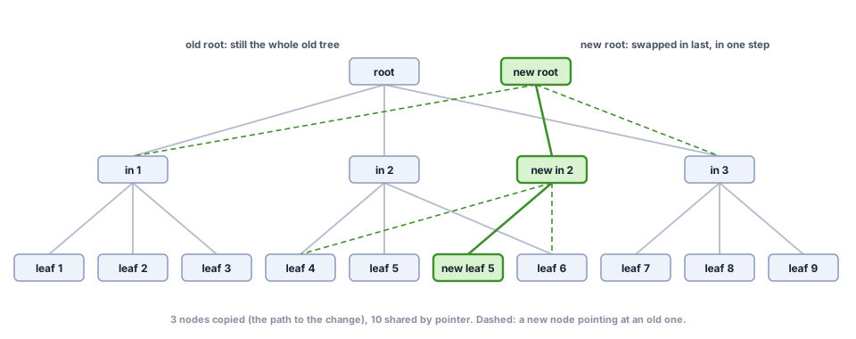
Only the path is copied. Copying a page means its parent must point at the copy, so the parent is copied too, and its parent, up to the root: exactly the nodes on the path from the change to the top, and nothing else. Every other node of the new version is the old node, reached by the same pointer. In the figure, one update copies 3 nodes and shares the other 10. In a B-tree three or four levels tall, every write copies three or four pages however many billions of keys sit below them. This is path copying.
The old version survives. Nothing reachable from the old root was changed, so the old root still leads to a complete, consistent tree: the one from before the update. Keep it and you can read that version for as long as you like. A structure that keeps its past versions readable is called persistent, and path copying is how search trees usually get there; LMDB keeps exactly two roots alive, the current one and the one being built. How far this goes has an honest edge. Keeping every past version readable is well understood for B-trees. Making every past version updatable as well, so that history can branch, was an open problem for them when Vitter surveyed the area in 2008 [28].
Readers need no lock. This one was stated above, and now it can be seen for what it is: a consequence of the other two, with no lock left to optimize. A reader holding the old root is reading a tree nobody will ever change, so there is nothing to protect it from.
The price is paid on writes. Every update rewrites a whole path rather than one page, and pages of old versions have to be reclaimed once no reader can still reach them, which is bookkeeping the update-in-place B-tree never needed.
Every design before the LSM-tree changed the structure to survive a fixed workload. The LSM-tree changes which operation gets to be cheap, because the workload itself, mostly writes instead of mostly reads, was the thing that broke.
2.9 ✎ Take a turn with the keys practice
Two kinds of work follow. First, eight projects: you build something, measure something, or explain something to another person. They have no single right answer, so nobody can mark them for you. After them comes a bank of numbered exercises, each with one right answer you can check. Do some of each: the exercises show what you know, the projects show what you can do.
Where a project needs code, let an AI write it; the times given assume it does. Your part is what the AI cannot do for you: saying what the code must do, building the check that shows it does, and judging what comes back.
Project 1 · hard · ~2 hours
Build a balanced tree. Have an AI write a binary search tree’s insert and lookup, then the red-black tree’s insert on top of it, using only the three repair moves (rotate left, rotate right, flip colors). Before you ask, write down what you will check: both trees agree on every lookup over the same random keys, and after every insert the red-black tree keeps its keys in order, keeps its root link black, obeys both red-link rules, and crosses the same number of black links on every path down. Build that check yourself. Then break one repair move on purpose, for instance a flip_colors that forgets to redden the node, and see which part of the check notices.
Project 2 · the binary search tree · ~45 min
Deliver what the tree promised. On your binary search tree, add min, max, floor and ceiling, then a subtree-size field on every node, and rank and select. The AI can write them; the checks are yours. Check that select(rank(k)) returns k again for every key you inserted, and that rank of a key you never inserted still returns a sensible count. Say what “sensible” means, exactly, before you run anything.
Project 3 · the binary search tree · hard · ~1 hour
Delete it two ways. Have an AI write both deletions from the binary search tree section: Hibbard’s copy the key, and move the node. Build two copies of the same tree, and in each hold a reference to the successor’s node before you delete the same two-children key. Afterwards, compare the keys and the shape: they agree. Then ask each copy where the node you held has gone: in one it is still in the tree, in the other it is not. Say what kind of program would notice the difference.
Project 4 · the binary search tree · hard · ~1 hour
Write the specification first. Before any code exists, write the contract for delete on an ordered dictionary: what it means (which key leaves, and what happens when the key isn’t there), which promise the tree must still keep afterwards, what it may cost, and what you fix exactly versus leave to whoever writes it. Hand only that to an AI and take the code it writes. Then look for a program that meets every line you wrote and is still wrong for you; Project 3 is one place to start. Name the line your spec was missing, and add it.
Project 5 · binary search tree against red-black tree · ~45 min
Pick the order that hurts. Your service keeps its users’ keys in a plain binary search tree, and the users choose the keys. Play the attacker first. Sorted order is the obvious attack, and the chapter has already shown it; find one that does not look sorted and hurts just as much, and measure what one lookup costs after a thousand keys arrive that way. Then write the guarantee the service needs as one sentence about cost, say which structure in this chapter delivers it, and say whether a guarantee that holds only on average, over random arrivals, would be enough here. An AI can write the measurement; the attack and the sentence are yours.
Project 6 · sorted array against tree · ~45 min
Change the workload, not the structure. Hold the same keys, inserted in random order, in a sorted array and in a binary search tree. Run a workload that is 90 percent inserts of new random keys, and one that is 90 percent lookups, first starting from a thousand keys and then from a million. Say which structure wins each run. If the winner of the insert-heavy run changes as the collection grows, find roughly where, and explain why it happens there. An AI can write the timing harness; you decide what it must hold fixed between runs, including how many operations run and how large the collection ends up. Measure it; do not reason it out. This is the one project here whose answer you are meant to get from a clock rather than from an argument.
Project 7 · hard · ~1 hour
Judge something you didn’t write. Take an ordered-collection implementation you had no hand in: a standard library’s sorted map, a database’s index, or whatever a model hands you when you ask for one. Don’t read it for correctness. Read it for its assumptions: which of this chapter’s structures is it, what does it take to be true about the workload, and what arrival order or access pattern would make it the wrong choice? Write those three down before you look at any documentation or ask an AI, then check. Most of the code you will ever depend on is code you did not write, and this is the only way to check it against what it promises.
Project 8 · ~20 min · no notes
Teach it back. Explain to somebody else why a B-tree’s nodes hold many keys while a red-black tree’s binary nodes hold one each. If you can’t name what changed about the cost of reaching a node, the explanation isn’t finished yet.
Here is flip_colors, written the way almost everyone writes it the first time:
def flip_colors(h):
    h.red = True
    h.left.red = False
    h.right.red = False
Every insert in this chapter still works. Every tree it builds is valid. Run a thousand random insertions and nothing complains, which is why this version gets published.
It was published, here. The defect is real: this version shipped in this book, and when a check was finally put in front of it, it corrupted 276 of 400 randomly built trees. The correct version had been sitting in the companion library all along, three directories away, under a test suite that was passing.
Three questions, in order, and do them in order:
- Before running anything, and without looking back (you met the answer in the red-black deletion section), say which of the two jobs
flip_colorsdoes in this chapter is the one this version cannot do, and name the caller that needs it. - Write the smallest input that tells the two versions apart: a key sequence, and the operation to run afterwards. Smallest means fewest keys. If yours has more than five, keep cutting.
- Now run it. Was your prediction in (1) right? Write down how confident you were before you ran it, then compare.
If you want to check your answer against a machine rather than against the book: the code printed in this chapter is tested against a companion library on every commit, and this exact defect is one of the cases that gate is required to catch.
Only after you have your own answer: hand the broken version to an AI and ask it to find the bug. Most will tell you the function looks correct, because it is correct: for insertion, which is the only context they can see in four lines. That is the lesson about where AI sits in this work. It cannot know what it was not shown, and you chose what to show it.
Everything above is worth more later than it is now, and the way to collect is to leave and return. Put this somewhere you’ll see it in about a week, and when you do, answer from memory first: no scrolling back, and no AI. Getting it wrong and then looking is the point; looking first isn’t.
- Name the six structures in order, and for each of the first five, the assumption that broke and forced the next.
- Draw the four-key tree that a sorted arrival builds, and say what a lookup in it costs.
- What are the two red-link rules, and what does each of the three repairs fix?
- A node holds a thousand keys instead of one. Which cost went down, which went up, and why is the trade worth it only sometimes?
- Something is written down but not yet filed, and the power goes out. What is lost, and what makes sure nothing is?
- A sign-up page checks “is this username taken?” with a Bloom filter in front of the user database, and says taken whenever the filter says “maybe”. Every test passes. What did the design assume, what one requirement would you add, and what test would have caught it? Check yourself: it assumed “maybe” means “yes”, so some free names are refused. The requirement: a name is reported taken only if the database holds it. The test: try names you know are free, and count how many come back taken.
Whichever of those you couldn’t reconstruct is the one to reread, and only that one. If you got all six, come back again in a month instead.
2.10 ✎ A bank you can mark yourself practice
Here are twenty-three exercises. Each shows roughly how long it takes, and everything you need for them is in the chapter so far.
If you only do four, do Exercises 4, 17, 21 and 22.
They are grouped by kind of task, not by structure. To practice one structure, here are the exercises for each section:
- Checking one place at a time: 1
- An orderly key ring: 2, 3, 23
- Escaping the line: 4, 5, 20
- Sticky red links: 6, 7, 8, 13, 14, 15, 16, 17, 18, 19, 21
- Frankenstein: 9, 10, 11, 22
- I’ll pay it back later: 12
2.10.1 Run it and report the state
Exercise 1 · gentle · ~5 min
Build a list that refuses duplicates by inserting 4, 9, 4, 2, 9, 7 one at a time, checking each key against the keys you have accepted so far, from the first, and stopping at a match. What does the list hold at the end, and how many key comparisons did the build cost?
Exercise 2 · gentle · ~5 min
Here is a sorted row of fifteen keys: 2, 5, 8, 11, 14, 17, 20, 23, 26, 29, 32, 35, 38, 41, 44. Binary search it for 14, and write down every key the search looks at, in order.
Exercise 3 · gentle · ~5 min
Here is a sorted row of fifteen keys: 2, 5, 8, 11, 14, 17, 20, 23, 26, 29, 32, 35, 38, 41, 44. Binary search it for 33, and write down every key the search looks at, in order.
Exercise 4 · gentle · ~10 min
Insert 60, 30, 80, 20, 45, 70, 90, 40, 50, 42 into an empty binary search tree. How tall is it, counting nodes (a single node has height 1)? What are ceiling(55), rank(43) and select(6), counting from select(0) as the smallest key?
Exercise 5 · middling · ~15 min
From the tree you built in Exercise 4, delete 30 by copying the successor’s key up into the node (Hibbard’s deletion, delete_hibbard in the companion library). Which key now sits where 30 was, and what hangs off it?
Exercise 6 · middling · ~25 min
Insert 75, 51, 79, 9, 36, 72, 40, 71, 70, 66, 4, 69 into an empty left-leaning red-black tree. Which keys have a red link into them?
Exercise 7 · middling · ~15 min
Starting from an empty left-leaning red-black tree, insert D, C, A, B, E, then F. After each insert, name every repair that fires (rotate left, rotate right, flip colors), in order, or say that none does. Letters compare in alphabetical order.
Exercise 8 · hard · ~20 min
Build the left-leaning red-black tree from 10, 20, 30, 40, 50, 60, then delete the smallest key twice in a row. Each time, say whether move_red_left fired, and at which node, and draw the tree afterwards.
Then: If the second deletion needed no push at all, explain what the first one left behind that made it unnecessary.
Exercise 9 · middling · ~15 min
Insert 17, 21, 8, 48, 27, 32, 11 into an empty B-tree of minimum degree t = 2, so each node holds at most 3 keys. What keys are in the leftmost leaf?
Exercise 10 · hard · ~25 min
Build the B-tree at t = 2 from 17, 21, 8, 48, 27, 32, 11, 7, then delete 27 and then 48. Draw the tree after each. Each time, say which of the chapter’s moves the deletion used: replacing the key with its predecessor or successor, redistributing a key from a neighbor, or merging two nodes. Then say what decided the move each time: where the key sat, and what its children or neighbors held.
Exercise 11 · middling · ~20 min
Give a B-tree room for three keys per node (minimum degree t = 2) and insert 1 through 20 in order. How many splits happen, how tall is the tree at the end, and how many nodes does a search for 17 fetch? Then count the same search in the plain binary search tree the same insertions build, and say the most any search can fetch in a perfectly balanced binary search tree of 20 keys.
Exercise 12 · middling · ~20 min
Keep the chapter’s list of where things are, allowing yourself three entries before a trip. In this order: the keys go in the hall bowl, the tickets in the desk drawer, then the keys move to your coat pocket, and the spare charger goes in the car; then the tickets move to your wallet, the spare charger is thrown away, the passport goes on the top shelf, and the umbrella goes by the door. Write out both sealed pages and the list exactly as they end up. Then answer “where are the keys?”, “where is the umbrella?” and “where is the flashlight?”, counting how many pages each question touched.
Then: The keys changed place before the first trip. Does Page 1 hold one entry for them or two, and why is that allowed when a page is never changed? Then say which of the three questions a Bloom filter on each page would have made cheaper, and by how many pages.
2.10.2 Which promise broke
These exercises are about the five rules of a valid tree: the keys are in order; the link into the root is black; a red link always leans left; no red link hangs directly below another; every path crosses the same number of black links.
First build the reference tree: insert 75, 51, 79, 9, 36, 72, 40, 71, 70, 66, 4, 69 into an empty left-leaning red-black tree. It is valid; check that before you go on.
Each exercise below is a tree an AI model returned after changing the insert code, claiming the tree still passes its checks. Build the tree and name every rule it now breaks.
Most are the reference tree with one thing changed. Three give you different keys or a different order; build what they say. Some changes only recolor a link; others move keys or change the tree’s shape.
One of these trees is valid. For that one, “nothing is broken” is the right answer.
Exercise 13 · middling · ~10 min
The model returns the reference tree with this changed: exchange the keys 70 and 72, touching no link and no color.
Exercise 14 · middling · ~5 min
A different tree, built from 20, 10, 30: repaint the link into the root (20) red.
Exercise 15 · middling · ~10 min
On the reference tree, apply rotate_right at the root (71), exactly as the repair code does.
Exercise 16 · middling · ~10 min
A tree of three nodes: a black link into 30, a red link into 20 as 30’s left child, and a red link into 10 as 20’s left child.
Exercise 17 · middling · ~10 min
On the reference tree, repaint the link into 51 from red to black.
Exercise 18 · middling · ~25 min
The same twelve keys, inserted in this order instead: 4, 79, 69, 71, 51, 9, 40, 75, 70, 72, 36, 66.
Exercise 19 · hard · ~15 min
On the reference tree, repaint the link into 69 from black to red.
Then: Count how many promises that one repaint took down, then say whether the count means the promises are badly chosen, or something else.
2.10.3 You supply the input
Exercise 20 · gentle · ~10 min
Make a plain binary search tree on the keys 1 to 8 as tall as it can possibly be. Give the insertion order. Then find a second order that reaches the same height but does not look sorted, and say what all such orders have in common.
Then: How many of the 8! possible orders of the eight keys reach that height? Guess first, then count.
Exercise 21 · middling · ~10 min
Now do the same to the left-leaning red-black tree: find an insertion order of 1 to 8 that makes it 8 tall, or as tall as you can. Predict what will happen before you run anything, and write the prediction down.
Then: State what you found as a sentence about insertion orders rather than about trees.
Exercise 22 · middling · ~25 min
Falsify this (find a case that shows it is false): two people who insert the same fifteen keys into a B-tree at minimum degree t = 2, in different orders, end up with the same tree. Then measure the height of every tree you built while falsifying it.
Then: Of the two things you checked, the tree’s shape and its height, say which a caller is entitled to depend on, which is not, and why the second is not a bug.
Exercise 23 · middling · ~10 min
Falsify this: binary search makes a sorted array beat the tree at everything, so the trees were never needed. Your answer has to name an operation and count something, not name a structure.
Then: State the workload under which the claim is actually true.
There are eleven more exercises later in the chapter. Ten come after the section that names the chapter’s nine core ideas, because most of them need those names. The last and hardest one is at the end of the appendix (Section 2.15.3), because it builds on the appendix.
2.11 ✎ When the ground shifts practice
Say you kept a sorted row of timestamps in memory and found things in it by binary search, halving between the two ends. Now the row is a log that keeps growing while you read it. You can still ask for the entry at any position, but nobody can tell you how many entries there are right now, and asking past the end just comes back empty. Binary search needs one thing it no longer has. Name it, say which idea in this chapter was built to search a sorted row without it, and say what it costs next to plain binary search.
A team is building a store for sensor readings: millions of writes an hour from tens of thousands of sensors, each reading keyed by its sensor and then its time, so writes land all over the key space. Readings are almost never read back, except as one sensor’s readings over a range of dates, and disk is the cheapest thing they have. A colleague proposes a B-tree, “because that’s what databases use.”
Name the assumption in that proposal this workload breaks. Say which structure you would argue for instead and, precisely, which cost you are agreeing to pay in exchange: which of read, update and space you are letting grow, since “it’s faster” names none of them. Then say what would have to change about the workload for your colleague to have been right all along.
2.12 ◆ What these are actually made of big picture
You just met six structures. That sounds like six things to remember. In fact they are built out of a handful of small ideas, used over and over in different combinations. The contracts chapter called those primitives. Here is every structure in this chapter, opened up.
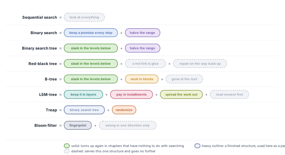
One thing to notice before the explanations start. The solid chips repeat; the dashed ones never do. Green, slack in the levels below, shows up in three rows running, because the same idea about slack is doing the work in the plain tree, the red-black tree and the B-tree alike. That repetition is the argument of this section, and it is visible before you read a word of what follows.
Sequential search = look at everything. No setup, no rules to keep, no promises. Every other structure in this chapter is an attempt to avoid doing this.
Binary search = keep it sorted + halve the range. Keep it sorted is a promise the structure keeps: true again after every change, even if an insert breaks it for a moment on the way. The search runs on a second promise, its loop invariant: if the key is anywhere, it lies between the two ends still being searched, working like a bookmark that always marks exactly what is left to read. Halve the range is divide and conquer: it is how you would guess a number between 1 and 100, never by starting at 1.
What changed: order, kept on purpose, lets one comparison rule out half of what is left.
Binary search tree = the same promise, kept in the shape instead. Slack in the levels below (a tree always has room underneath): writing a name into a sorted paper list pushes everyone below it down a line; a filing tree has an empty slot already hanging there. And halve the range again, now built into the shape.
What changed: order moved out of the positions and into the shape, so an insert no longer shoves anything.
Left-leaning red-black tree = the tree + a promise about its shape. Slack in the levels below, as before; a red link is glue, so two nodes joined by one count as a single node holding two keys; and repair on the way back up: three small fixes, each handling one bad shape, applied at every node on the way back from an insert. Nothing is ever rebuilt from scratch.
What changed: the shape now has a promise of its own, so the height stays short whatever order the keys arrive in.
B-tree = the same tree, with the nodes made fat. Slack in the levels below, a third time; work in blocks (block decomposition): a library is shelved into labeled sections, and walking to the shelf is the expensive part while scanning it is nearly free; and grow at the root, the only way for a tree to get taller while keeping every leaf at the same depth.
The algorithm stayed the same. What changed is what you are being charged for. If moving to the next node is as cheap as comparing two keys, comparisons are what you pay for. If moving to the next node means fetching it from somewhere slower, the fetch is what you pay for, and every fetch brings a whole block of neighboring keys along, whether you wanted them or not. A disk works that way, one page at a time. So does ordinary memory, one cache line at a time. Change the price list and a different structure wins, with no new idea needed.
LSM-tree = stop repairing, start stacking. Keep it in layers (layering): express and local trains, a small fast layer in memory in front of large slow ones on disk. Pay in installments (amortization): never do the big merge when a write arrives, but charge it to the many writes that caused it, the way a monthly subscription spreads one large cost over many days. That is a promise about the average, and it says nothing about the one write that happens to trigger the merge. Spread the work out (deamortization): do the merge itself in small pieces, in the background, off the write’s path, so no single write waits for all of it. That works only while the background keeps up. If writes keep arriving faster than it can merge them, the unmerged pile grows until the engine has to make new writes wait; RocksDB calls this a write stall. Spreading the work out removes the spikes, not the work. Read newest first: nothing is ever overwritten, so always believe the newest copy, and that one rule is what makes it safe never to overwrite anything.
What changed again is the price list. This time writes became the expensive direction.
Two more, each one idea bolted onto something you already have:
- Treap = binary search tree + randomization. Shuffle a deck before dealing and no one can stack it against you. Give each key a random priority and the arrival order stops being something an opponent can exploit. The frontier map after the chapter’s ending takes it further.
- Bloom filter = fingerprinting + agreeing to be wrong in one direction only. Compare two long documents by their checksums instead of line by line. It may say “maybe present” when the key is absent, never “absent” when it is present. Allowing the first mistake is what makes it tiny; refusing the second is what makes it safe to skip a file.
2.12.1 Choosing one, under pressure
This is the table to have in front of you when somebody needs an answer this afternoon. Every structure makes a promise, and two different things can go wrong with it. Break what the promise needs, and the promise is simply false. Break what makes the structure a good choice, and the promise still holds, but you are paying for the wrong thing. In the good-choice column, the last condition in each row is the one the next structure was built to fix.
| structure | the promise needs | it is a good choice when | what keeping it costs |
|---|---|---|---|
| Sequential scan | nothing | the collection is tiny, or searched only once | nothing |
| Sorted array | the keys are sorted | comparing keys is cheap, and the collection rarely changes, because every insert shifts the row | shifting the row on every insert |
| Binary search tree | at every node, smaller keys on the left and larger ones on the right | comparisons are cheap, and keys arrive in mixed order, because sorted arrival grows one long line | nothing |
| Red-black tree (LLRB) | its five promises are restored after every insert and delete | the height is worth a small repair on every change, and reaching any node costs about the same as reaching any other | a repair on every insert and delete |
| B-tree | every node but the root is between half full and full, and all leaves sit at the same depth | reaching a node costs far more than comparing the keys inside it, and a write can afford to go straight to the one place its key lives | fat nodes, each about a third empty |
| LSM-tree | every write is logged first, finished files are never edited, and a read believes the newest record it finds | writes arrive faster than reads, a read can afford to look in several places, and there is spare time later to merge files | merging later, and the write amplification it costs |
Almost every row is the right answer for somebody, and none of them is the right answer for everybody. The contracts chapter gave that shape a name: the rows are non-dominated, meaning no other row is at least as good on every cost and better on one. The one exception comes with the numbers, below.
That table is what I draw at a whiteboard. The one below, with the numbers, is the one I look up.
2.12.2 What each one costs
Worst case throughout, for \(n\) keys. \(h\) is the height of a tree nobody is keeping balanced, which is anywhere between \(\lg n\) and \(n\). \(t\) is the B-tree’s minimum degree, defined under “B-tree height”. rank and select cost the height only on a tree whose nodes each carry a count of the keys below them, which is one more field per node than the space column lists.
| structure | search | insert | delete | min/max, floor/ceiling, rank/select |
extra space per key |
|---|---|---|---|---|---|
| Sequential scan | \(\Theta(n)\) | \(\Theta(1)\) to append, \(\Theta(n)\) to check first | \(\Theta(n)\) | \(\Theta(n)\) | none |
| Sorted array | \(\Theta(\lg n)\) | \(\Theta(n)\) | \(\Theta(n)\) | \(\Theta(\lg n)\); min/max and select are \(\Theta(1)\) |
none |
| Binary search tree | \(\Theta(h)\) | \(\Theta(h)\) | \(\Theta(h)\) | \(\Theta(h)\) | two links |
| Red-black tree (LLRB) | \(\Theta(\lg n)\) | \(\Theta(\lg n)\) | \(\Theta(\lg n)\) | \(\Theta(\lg n)\) | two links, one bit |
| B-tree | \(\Theta(\log_t n)\) fetches | \(\Theta(\log_t n)\) fetches | \(\Theta(\log_t n)\) fetches | \(\Theta(\log_t n)\) fetches | each node up to half empty |
Five things the table is telling you that its numbers do not.
Every tree row reads the same across. Search, insert, delete and all six ordered questions cost the height, because all of them are the same walk wearing different hats: one comparison per node, height many nodes. That is why every tree in this chapter was judged on height and nothing else.
One row is beaten outright. In every time column the red-black tree’s bound is no worse than the plain binary search tree’s, and its worst case is strictly better, which is what the contracts chapter called domination. The plain tree is here because you have to build one before the repairs make sense; you would not ship one. The space column softens it: the plain tree carries no color bit and pays nothing on the way back up. The axes were a choice here too.
The ordered questions are the reason to be here at all. On a typical search a hash table beats every row in this table, though not in the worst case. What it cannot answer is a single thing in the fifth column, because throwing the order away is how it got its speed. If you never need that column, use a hash table and skip all of this. Everything here is the price of keeping order.
The sorted array’s split personality is the chapter’s opening lesson, in one cell. select is free because position is rank. That is the same fact that makes insert cost \(\Theta(n)\). One fact, one gift, one wound.
The LSM-tree has no row in this table, and that is the honest answer. A write costs one in-memory insert, with no disk seek. A read costs more than any formula in \(n\) says: it depends on how many levels you let pile up, how much you compact, and whether a Bloom filter sits in front. It is a dial you set rather than a bound you inherit, and anyone who hands you a single formula for it is selling something.
2.12.3 The same nine ideas, over and over
Read down this table, not across it.
| primitive | where else it turns up |
|---|---|
| keep a promise every step | Dijkstra’s settled set, insertion sort |
| halve the range | mergesort, the fast Fourier transform |
| slack in the levels below | AVL trees, skip lists, heaps |
| work in blocks | disk pages, cache lines |
| keep it in layers | skip lists |
| pay in installments | a growable array, union-find |
| spread the work out | a hash table that resizes a little at a time, a real-time queue |
| randomize to dodge the worst case | quicksort’s pivot, hash tables |
| fingerprint instead of comparing | checking files match, Karp-Rabin |
Nine ideas, six structures, and every one of those ideas turns up again in chapters that have nothing to do with searching.
That is why this list is worth more than the six structures were. When a workload arrives that matches nothing in the table, you are not stuck hunting for a name you recognize. You ask what it costs, which promise is worth keeping, and which of these ideas pays for it, and then you build the thing that does not have a name yet.
2.12.4 Which idea do you reach for
Each of these nine exercises describes a situation, most of them new to this chapter, and asks which of the nine ideas above you would use. Each idea is the right answer to exactly one of them.
Exercise 24 · middling · ~5 min
A messaging service keeps, for every conversation, the messages in time order. Reads ask for the newest few. Writes arrive in bursts, far faster than reads, and a message is never edited once sent. Which idea do you reach for first?
- slack in the levels below
- keep it in layers
- work in blocks
- fingerprint instead of comparing
Then: Name the failure mode you just bought, in this chapter’s terms.
Exercise 25 · gentle · ~5 min
A read-only dataset of 40 million records ships once a month on a disk image and is loaded into memory on arrival. Every query is a lookup by id, or asks for all records whose ids fall between two bounds. Nothing is ever inserted between shipments. Which idea do you reach for first?
- slack in the levels below
- keep it in layers
- halve the range
- pay in installments
Then: What single change to this workload would make your answer wrong?
Exercise 26 · middling · ~5 min
A service must answer “have we seen this id before?” for a stream of billions of ids, in memory that holds only a small fraction of them, where a wrong “yes” costs one wasted lookup and a wrong “no” corrupts the records. Which idea do you reach for?
- fingerprint instead of comparing
- work in blocks
- keep a promise every step
- randomize to dodge the worst case
Then: Errors here have two directions. Say what your choice does to each of them, and why that matches this workload.
Exercise 27 · hard · ~10 min
An index is a plain binary search tree, and its keys are ids chosen by whoever is calling. One caller has worked out that a particular arrival order makes every lookup slow. You cannot change the tree’s code, because it is a library you depend on. You can change only the order in which keys are handed to it: the index is rebuilt from scratch every night from the full list of ids, and you may reorder that list before passing it on. Which idea do you reach for?
- slack in the levels below
- halve the range
- randomize to dodge the worst case
- work in blocks
Then: Compare the guarantee you just bought against a balanced tree’s, in one sentence.
Exercise 28 · middling · ~10 min
A sorted array is the right structure for a read-heavy index, but a few hundred inserts a day do arrive, and each one shoves a large part of the array along, stalling the service for a visible moment. The total work is affordable; it is the spikes that are not. Which idea do you reach for?
- pay in installments
- halve the range
- spread the work out
- keep a promise every step
Then: Name a workload where this is the wrong trade, and say what about that workload makes it wrong.
Exercise 29 · middling · ~5 min
An in-memory red-black tree holds a hundred million keys. A profiler says lookups spend nearly all their time waiting on memory rather than comparing: almost every node visited is a cache miss, and each miss brings in a whole cache line, typically 64 bytes, of which the node uses a fraction. Nothing moved off the machine. Which idea do you reach for?
- halve the range
- work in blocks
- randomize to dodge the worst case
- keep a promise every step
Then: Name the block here, and say why a disk or a network round trip would have led you to the same idea.
Exercise 30 · middling · ~5 min
An in-memory index must support lookup, ordered iteration, and range queries, with reads and writes in about equal numbers. The keys are timestamps from thousands of sensors whose readings arrive late: each sensor’s keys come in increasing order, but a new key can land anywhere in the range already stored. You control the structure entirely. Which idea do you reach for?
- halve the range
- keep it in layers
- slack in the levels below
- fingerprint instead of comparing
Then: Say why each of the three wrong answers fails here.
Exercise 31 · hard · ~10 min
You add a subtree-size field to every node so the tree can answer rank and select. Insert maintains it. A colleague now adds a delete, and a bulk-load path that builds nodes directly. What makes the field safe to read?
- keep a promise every step
- pay in installments
- work in blocks
- randomize to dodge the worst case
Then: This is the same risk the broken trees in Exercises 13 to 19 showed: a promise that holds only until a new code path touches the nodes. Say why.
Exercise 32 · middling · ~5 min
A nightly batch job appends a hundred million log events to a growable array that doubles its capacity whenever it is full. The job is judged only on when the whole run finishes; nobody waits on any single append. A reviewer objects that some appends copy the entire array. Which idea says the objection does not matter here?
- pay in installments
- spread the work out
- work in blocks
- slack in the levels below
Then: Change one thing about the workload that would make (b) the right answer instead.
2.12.5 The tests pass. What did they miss?
Code that fails its tests is easy to catch. The costly kind passes every test, because nobody wrote a test for the requirement it breaks.
Exercise 33 · hard · ~20 min
A colleague’s key-value store is an LSM-tree: writes go into a memtable, a full memtable is flushed to a sorted file that is never edited again, deletes write tombstones, reads go newest first, and compaction merges files in the background. Three tests guard it, and all three pass: after any random sequence of writes and deletes, every read agrees with a plain dictionary given the same sequence; the same holds after every compaction; and every file on disk is sorted and unchanged once written. In its first week the machine loses power. The store restarts cleanly and every file is intact, but the last few hundred writes the service had confirmed to its callers are gone. Name the requirement the tests never stated, and write it as one sentence a test could check.
Then: Describe the test that would have failed, then say what the store must do to pass it and what that costs on every write.
2.12.6 Fill in the card
No options this time. The workload below is not one of the chapter’s, and the answer is not a name: it is seven short answers, the same seven the B-tree got in “The B-tree, question by question”.
Exercise 34 · hard · ~40 min
A weather network has thousands of stations, and together they send tens of thousands of readings a second, all day. Each reading must be confirmed to its station within ten milliseconds, every time, even in the busiest minute of the year, and a confirmed reading must never be lost, even in a power cut. Reads are rare: a weekly report per station, and now and then a look at one station over one afternoon, and nobody minds if that takes a few seconds. Answer the seven questions from the contracts chapter for this workload, one or two sentences each.
Then: This workload makes three separate promises. Name them, name the idea that keeps each one, and say which of the three costs something on every single write.
2.13 ◆ Where that leaves the keys big picture
Start to finish, this chapter did one thing over and over. It took a structure that worked, found the assumption holding it up, and then changed the world until that assumption broke. The table in “Choosing one, under pressure” is that story, one row per structure.
One exception is already named: on the time bounds in “What each one costs”, the red-black tree beats the plain binary search tree. Apart from that, not one of those structures is better than the one before it. Each is the same trade made against a different assumption about the world, and every one of them is still the right answer somewhere today. A sorted array is exactly right for data that never changes. A plain binary search tree is fine when the keys arrive shuffled. Wide nodes are wasted wherever reaching a node is as cheap as comparing a key, and win wherever reaching one is the expensive step: on disk by a mile, and in memory, one cache line at a time.
Which is why the most useful thing to carry out of here is the habit of asking, before choosing one, what this workload actually costs: what’s cheap, what’s expensive, how often things change, and whether anyone will ever need the keys in order. Answer that honestly and the ladder tells you where to stand on it. Answer it wrong and you’ll have built something beautiful for a problem nobody has.
One last note about words, so none of this is stranded here. Almost everything this chapter named is what the rest of the world calls it too: node, root, leaf, child, parent, subtree, 2-node, 3-node, rotation. Walk into any room where this material is spoken, open any implementation, ask any model, and those words will be waiting, now meaning something.
Three were this chapter’s own and stop at its edge. Glue for a red link, an armful for what one block fetch buys, a spare red link: useful here, unknown elsewhere. They were scaffolding for the ideas underneath, and the ideas keep their standard names: a red link inside a 3-node, a block, a borrowed red link. The hook was scaffolding too, and it did its job at the top of the chapter: a node is a thing you hang a key on, which is all you ever needed the picture for.
These six structures are a table of contents for half the data-structures literature.
The keys were never really the point. Knowing what it costs to find them was.
2.14 ★ Frontier map advanced
What follows is optional: a short tour of a few ideas sitting just past the edge of this chapter, not the next step in this chapter’s sequence. Skip it now if you’d rather move on, and come back to it later.
2.14.1 What order costs, proved
Predecessor lower bound
The chapter has one lower bound already: a search by comparisons needs about \(\lg n\) of them, because each answers yes or no. Hashing steps around it by not comparing at all, and for “is this key present” it wins outright: a hash table built for a fixed set of keys can answer in a constant number of steps, in the worst case, in space proportional to the keys [29]. So the fair question is whether that escape works for the ordered questions too. Can some cleverer arrangement of machine words answer “what is the largest key at or below this one” in constant time, if it is allowed to compute on the keys’ bits instead of comparing them?
Not in general, and this time the answer is a theorem rather than a failure to find something. In a model that charges only for reading memory and lets every other computation be free, the number of reads predecessor search needs is known exactly, up to constant factors, for every combination of key count, key length and space [30]. It is constant only at the extremes: keys so short that a table with one slot per possible key fits in the space, or machine words so long that one of them holds a large fraction of the keys. Everywhere between, with space not much larger than the keys, it is not constant: it grows with the number of keys, their length, or both, depending on how much space there is. The van Emde Boas tree comes close to it for some of those combinations, taking about \(\lg w\) steps for \(w\)-bit keys by searching over the bits of the key rather than over the keys. Membership is constant; predecessor, between those extremes, is not and cannot be. That is the precise price of the order this chapter has been paying to keep.
The bound holds unconditionally: no unproved conjecture is holding it up. That is rarer than it sounds. Many “we cannot do better” statements in this subject hold only if some widely believed conjecture is true, and the same kind of reasoning about memory reads is still producing new unconditional bounds for problems whose data keeps changing [31]. When someone says an algorithm cannot be improved, the first question is which of the two kinds of claim they are making.
Signature: someone promises constant-time ordered queries, the next key or a range, on arbitrary keys. Reach for this bound to ask what they are assuming: keys so short a table covers them all, machine words long enough to hold many keys, or far more space than the keys themselves.
2.14.2 The best possible tree, when you know what gets asked for
Optimal binary search tree
Every tree in this chapter treats its keys as equally likely to be wanted. Real workloads don’t. Given \(n\) keys and a known access frequency for each one, there is a provably best static tree: the one minimizing total frequency-weighted search cost. Not the shortest tree, and not whatever a run of random inserts happens to produce: the actual optimum for a known query pattern.
A greedy rule won’t find it. Compression codes, where a similar-looking tree problem is solved greedily, get away with it because there every item hangs at a leaf, so the tree is free to put the frequent ones nearest the top in any arrangement it likes. A search tree can’t: its keys sit at every level, and the ordering property fixes which key may go where.
Finding it needs dynamic programming: \(O(n^3)\) time, trying every possible root for every contiguous range of keys. It drops to \(O(n^2)\) because of something Knuth noticed: add a key on the right of a range and the best root never moves left; add one on the left and it never moves right. So each range’s best root lies between the best roots of its two slightly shorter neighbors, and the search only tries the keys between those two, instead of scanning the whole range again [32], [33]. Yao later traced that monotonicity to a more general condition on the costs, the quadrangle inequality, which speeds up a whole family of dynamic programs the same way [34].
Signature: a workload where a small, known set of keys takes most of the traffic. Reach for it when the frequencies are stable enough to be worth measuring, and note what it gives up, which is every kind of change. It is a static structure, in the sense defined under self-adjusting and learned structures below.
2.14.3 Cost trade-offs and the RUM conjecture
The RUM conjecture
A good trade-off doesn’t try to make every cost equal. It spends more of whichever resource is cheap in order to save a larger amount of whichever resource is expensive. The B-tree is the clearest example already in this chapter, and the striking thing is what it does not attempt: nobody designing it is trying to bring the cost of reaching a node and the cost of comparing a key into line with each other. The design deliberately widens the gap between them instead, spending comparisons without counting, precisely to avoid paying for one more access.
The shape has a name you have already met, boxed in the LSM-tree section: the RUM conjecture, under which an index can make two of its read, update and memory overheads small only by letting the third grow. The B-tree and the LSM tree sit at two of its corners.
The same shape shows up earlier in the chapter too. The red-black tree spends a little extra comparing and rotating on every insert specifically to avoid the far more expensive cost of a lookup walking down a degenerate, sequential-search-shaped tree. Sortedness itself is a trade: the sorted array spends a shifting cost on insertion to buy a cheap halving cost on every search after it. None of these structures are balancing their costs; each one is choosing, deliberately, which cost to make cheap and which cost to make rare. Whenever one operation is far more expensive than another, the right structure spends the cheap one freely, without hesitation, to avoid the costly one.
Hashing takes this trade-off to its end, and it earns its place honestly: \(O(1)\) average-case lookup beats anything a tree in this chapter can offer. But it buys that speed by giving up the one thing every design here was built to keep, which is order. A hash table cannot answer “what is the next key after this one,” or “give me everything between these two bounds,” without looking at every key it holds. The order it threw away was the thing that made those questions cheap. Whether that trade is the right one depends entirely on whether an application ever asks an ordered question. Plenty never do, and for those, everything in this chapter is overhead.
2.14.4 Self-adjusting and learned structures
Splay tree, treap, skip list, learned index
Everything built so far is one of two kinds: built once and left alone, or kept correct across changes, which is what dynamically maintained means here. There’s a step past dynamically maintained, and a further step past that.
Static. The clearest example is a sorted array you build once and never insert into again: a workload assumed to hold still, with no invariant to maintain because nothing ever changes after it’s built.
Dynamically maintained. Every structure in this chapter (the sorted array included, the moment it starts taking inserts) keeps some invariant true across changes: sortedness, left side smaller and right side larger, the two red-link rules, a sorted run of keys inside every node. An insert may disturb that invariant for a moment, but the structure puts it right again before the insert is allowed to finish.
Self-adjusting. A splay tree [35] goes one step further: every access, even a lookup that changes nothing, reshapes the tree, using the same rotate left and rotate right already familiar from the red-black tree, to walk the node just reached up toward the top.
Three named moves do the walking. Which one fires is decided by where the node sits relative to its parent and grandparent, and by nothing else:
- zig: the parent is the root. One rotation, and the walk is over.
- zig-zig: node and parent lean the same way. Two rotations, which fold the whole chain upward together.
- zig-zag: node and parent lean opposite ways. Two rotations, which straighten the kink before lifting.
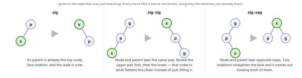
The middle one carries the whole idea. A naive “rotate it up until it reaches the top” would also put the node at the top, but it would leave the long chain it climbed almost as long as it found it. Rotating the upper pair first folds that chain in half on the way past, which is why a splay tree gets faster over a run of accesses and a naive lift does not.
Keys reached often end up close to the top on their own, keys rarely touched drift down, and there’s no colored link and no rule to check or repair; the shape adjusts itself purely from which keys get used.
Splay trees also carry one of the oldest open questions in the subject. Their inventors conjectured that over any long run of accesses a splay tree is within a constant factor of the best binary search tree that knew the whole run in advance and could rearrange itself for it [35]. That conjecture is still open. For decades the best anyone could prove for an adapting tree was a different design, the tango tree, within a factor of \(O(\lg \lg n)\) of that best [36], while for splay trees themselves nothing better than a factor of \(\lg n\) was known. In July 2026 splay trees were shown to be within a factor of about \(\lg \lg n\) as well, up to smaller terms [37]: close, and still not the constant the conjecture asks for.
That self-adjusting trick carries three costs worth naming together, because the next idea is a direct answer to them [38]. Restructuring the whole path to the top happens on every access, even a plain lookup that found what it wanted and changed nothing. A single one of those restructurings can still take as many rotations as the tree is deep. And the guarantee that makes splay trees famous is an amortized one: it promises that a long run of operations is cheap on average, and says nothing whatsoever about the operation you are waiting on right now, which does not help at all if the thing waiting is a request with a deadline.
Randomized. A treap answers that critique with a different trade: give every key, alongside its place in the order, a second number picked at random when it’s inserted, its priority, and keep the tree simultaneously a binary search tree on keys and a heap on priorities, the larger priority always sitting above its children [39]. For any fixed set of key–priority pairs there’s exactly one tree shape satisfying both rules at once, so insert as an ordinary node, then rotate it upward only while its priority beats its parent’s, and there’s never a real choice about where it ends up. Because the priorities are random rather than chosen, an expected constant number of rotations, two on average, settles every insert or delete, and the tree stays within a constant factor of balanced with no colored link and no repair rule to maintain [38]: the red-black tree’s promise kept by chance instead of bookkeeping, and so kept on average over the coin flips, for every arrival order, rather than in each tree it builds.
A skip list spends the same coin on a different shape [40]. Drop the tree entirely and keep an ordinary sorted chain of keys, then, above it, a second chain holding a random half of them, and above that a chain holding a random half of those, and so on up. Searching starts on the sparsest chain at the top and walks forward until the next key overshoots, then drops one level and walks forward again, so each level cuts the remaining stretch roughly in half: the same halving the tree does, laid out sideways. Nothing in a skip list is rotated, recolored or repaired: a new key flips coins to decide how many levels it appears on, and that is the entire balancing discipline. The result is within a constant factor of \(\lg n\) with high probability, and the structure is far easier to make safe for many threads at once than any tree that rearranges itself, which is why skip lists turn up inside databases and in-memory stores. The randomization that makes this work is a subject of its own, and the skip list gets its full treatment there, alongside the other structures built out of coin flips, rather than here.
Learned. A learned index gives up walking node to node at all. Train a function, on the keys already present, that guesses roughly where any query key should sit in a sorted array [41]. Probe that guessed spot directly, and if it’s wrong, don’t fall back to a blind halving search: step outward from the guess, doubling the stride each time, then finish with an ordinary binary search once the true position is bracketed between two probes. A guess that’s off by \(\eta\) positions costs at most about \(2\log_2 \eta\) probes to recover from [42]. The guess replaces the walk through explicit structure; the correction step is what keeps it from ever being trusted blindly.
Put real numbers on that, because the bound is more demanding than it first sounds. Half a million keys, sorted. Plain binary search finds any one of them in at most 19 probes. Now let the model guess, and suppose it lands within 400 positions of the truth: step out 1, 2, 4, and on up to 512 to bracket the answer, about 10 probes, then binary-search the bracket, about 8 more. Call it 18, against binary search’s 19. All that machinery, to save a single probe.
Push the guess to within 10 positions and it costs about 7 probes, a genuine win. Let it drift to 2,000 and it costs about 22, which is worse than the plain halving search it replaced. The crossover is worth doing in your head: \(2\log_2 \eta\) beats \(\log_2 n\) exactly when \(\eta < \sqrt{n}\). For half a million keys that is roughly 707 positions. A learned index is a bet that the data’s shape is regular enough to predict a position to within the square root of the collection’s size, and the correction step is what makes losing that bet survivable rather than fatal.
That was the proposal, and the setting it was first made for is keys that sit still and are only read. Keys that arrive and leave while the index is being read are a harder setting, and practitioners stayed wary long enough that the first broad measurement was an event of its own: updatable learned indexes against each other and against ordinary trees, on ten real datasets, under changing key distributions and many threads at once, judged on speed, on memory, and on robustness [43]. On one thread the newer learned indexes won in over 80% of the settings tried. With many threads, some of the design choices that made them fast turned out to be at odds with keeping them safe to share, and they got slower. Its title asks whether they are ready, which is the right question to ask of any structure that is fast on the benchmark it was introduced with.
Robustness is on that list for a reason, and it is the reason worth carrying away. A learned index models the distribution of the keys, so whoever controls the keys controls the structure. Every implementation shares this weakness, because it is the mechanism working as designed, turned against you. Insert keys chosen to be awkward for the model, and the model has to spend more of itself describing them: poisoning 10% of the keys fed to one well-regarded learned index made it up to 120 times larger [44]. On another, which adapts its model as keys arrive, a stream of adversarial inserts slowed lookups by up to 2.8 times, while poisoning the keys it was first built from did little [45]. The balanced trees in this chapter keep their bound for every sequence of keys, so there is no lever of that kind on them. Written as a contract, the learned index’s assumption field says what the numbers above only implied: the keys follow a shape the model can learn, and nobody is choosing them against you.
Each step hands more of the work of positioning a key over to something other than fixed, hand-written rules: first to a rule that repairs itself, then to the pattern of use, then to chance, then to the data’s own shape.
Signatures, one each. A splay tree: a few keys take most of the traffic, nobody knows in advance which, and an occasional slow operation is acceptable. A treap or a skip list: the balanced tree’s bound, in expectation, with the least code, when nobody choosing the keys can see your coin flips, and the skip list especially when many threads share the structure. A learned index: keys that change rarely and follow a shape a model can learn to within about the square root of the collection’s size, chosen by nobody working against you.
2.14.5 Trees that can prove what they hold
Merkle tree
So far you have always been the one holding the structure. Suppose you are not. Suppose the index lives on somebody else’s machine, you ask it for one key, and it hands back an answer. How would you know it was not simply made up?
An authenticated, or Merkle, tree answers that by storing, at every node, a hash of the nodes beneath it. The single hash at the top is then a fingerprint of the entire contents: change one key anywhere and every hash on the path up to the top changes with it. To convince you that some key really is in there, the server sends only the key, plus the handful of sibling hashes along the path from that key to the top, about \(\lg n\) of them, and you recompute your way upward and check that you land on the fingerprint you already had.
That is the fingerprint primitive from the Bloom filter, put to a different job. There it bought size; here it buys trust, and the trade is the same shape: a small thing standing in for a large one, on terms you can state exactly. The durable idea is the one this chapter has been circling from another direction (verify, rather than trust), and it is what makes these trees the backbone of version control, of certificate transparency logs, and of every distributed ledger you have heard about.
Signature: the data sits on a machine you do not trust, and every answer has to come with evidence you can check against a small fingerprint you keep yourself.
2.14.6 Search without a map
Navigable small-world graphs
The skip list a few pages back searched in a way worth pulling out on its own. At every point it knew only the links leaving the key it stood on, and it took whichever link got it closest to the target without overshooting. No global picture, no plan: one greedy step at a time, and the levels guaranteed that a step always existed which cut the remaining distance by about half.
Now take away the levels and keep only the greedy walk. A collection of points, each linked to a few others, and a search that moves, at every step, to whichever neighbor is closest to the target. When does that work?
The obvious answer is “when short paths exist,” and it is wrong. Link each point to a handful of others picked uniformly at random, and short paths exist between everything: a random graph like that has paths of about \(\lg n\) links between any two points. Greedy search cannot find them. From where it stands, a link to a random point is almost always a link to somewhere far away, and none of those far links knows anything about the neighborhood of the target, so the last stretch has to be walked step by step. Short paths existing and short paths being findable are different properties.
Kleinberg found exactly what the second one needs [46]. Put the points on a grid, link each to its grid neighbors, and give each one extra long link, landing at distance \(d\) with probability proportional to \(d^{-r}\). On a two-dimensional grid, greedy search finds short paths when \(r = 2\), and for every other exponent it needs a number of steps that grows as a power of \(n\). The good exponent is unique, and it equals the grid’s dimension: at that value, every scale of distance gets about the same share of long links, so wherever the search stands, some link leads roughly halfway to the target. That is the skip list’s promise again, arrived at from the other side.
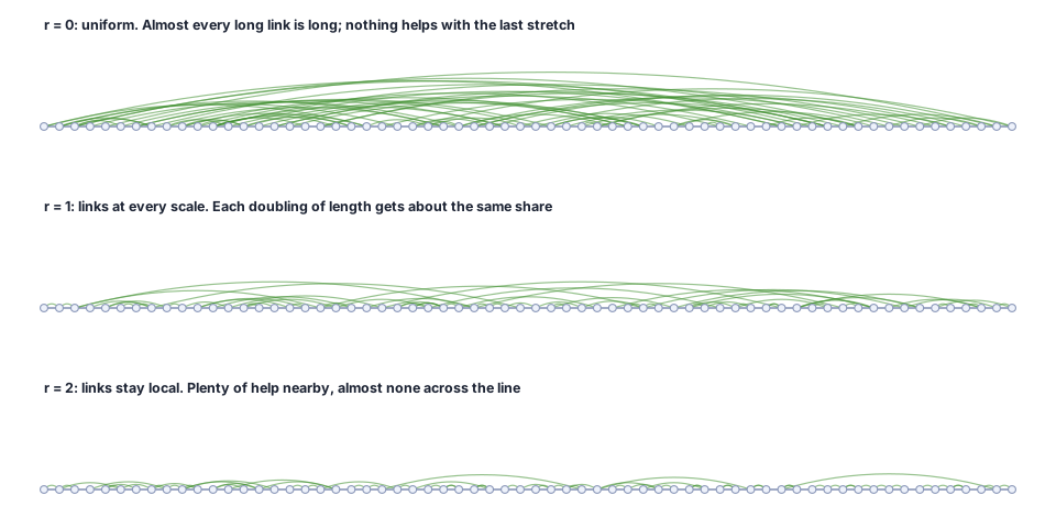
A ring has one dimension, so on a ring the good exponent is 1, not 2. The difference only shows at size. On a ring of points with one long link each, averaging 300 greedy searches between random pairs (measured 2026-09-29, book/figures/gen_navigability.py --table):
| points | uniform, \(r = 0\) | \(r = 1\) | \(r = 2\) |
|---|---|---|---|
| 1,024 | 28 steps | 22 | 118 |
| 16,384 | 119 | 53 | 1,339 |
| 262,144 | 444 | 91 | 16,656 |
Multiply the points by 256 and the uniform ring’s searches get about 16 times longer, the local ring’s 141 times. The ring whose exponent matches its dimension gets about 4 times longer.
The same construction keeps being found independently. Chord, a lookup scheme for machines on a network, places machines at identifiers on a ring and gives each one links to the machines responsible for the identifiers \(1, 2, 4, 8, \ldots\) ahead of its own: one link at every scale, exactly [47]. HNSW, the index behind much of today’s search over embeddings (lists of numbers standing for texts or images, where nearby lists mean similar things), stacks graphs of points in the way a skip list stacks its chains, and its authors describe it by that analogy [48]; the metric skip list is one of the standard structures for exact nearest-neighbor search [49].
The honest half comes in three clauses. Links alone buy short paths. The right links buy paths a greedy search can find. And being findable costs space: the sparsest graph on which greedy search always reaches its target can need on the order of \(n\sqrt{n}\) edges in the worst case, which is one reason deployed indexes aim only at being almost navigable [50]. What that costs is measurable too: for several popular indexes there are inputs on which a query takes a number of steps linear in the size of the data before it reaches any of its true nearest neighbors [51]. Where the data has few effective dimensions, the guarantees are much better [52], and that assumption belongs in the contract of any index built this way.
Signature: nearest-neighbor search over points with many dimensions, where there is no order to halve. Reach for it when a near answer is acceptable and the data has few effective dimensions.
2.14.7 Taken further: removing the last lock
Bw-tree
Copy-on-write frees the readers, and leaves one writer at a time rebuilding a path. The Bw-tree goes the rest of the way [53]. A node is never rewritten, not even as a copy: an update is appended as a small record describing the change, chained in front of the node, and nodes are reached through a table of addresses that each writer updates with a single atomic compare-and-swap, one hardware instruction that replaces a value only if it still holds what the writer last saw, so many writers can proceed at once without anyone holding a lock. Old records are freed only once no thread can still be looking at them. Read it beside the report of a second team that built one from the published description and recorded how much the description had left out, and how much tuning its speed depended on [54]. Proposal, then measurement: the same shape as the learned index above, and the same lesson: read the measurement, not only the proposal.
Signature: many threads writing the same ordered index at once, where a lock on the hot path is the bottleneck. Reach for it with the second team’s measurements in hand.
2.14.8 Could the whole chain choose itself?
Every design in this chapter got chosen by hand: look at the problem, look at the workload, look at the hardware’s limits, then pick a representation and an algorithm to match. Could that whole chain run itself one day, choosing its own structure the way this chapter chose one, step by step, without a person first walking through what each candidate takes for granted? Pieces of this already exist: a query optimizer picking a plan for a stated workload, autotuning that searches over implementations for a given machine, a learned index inferring its own guess straight from the data. But no single mature system yet runs the process end to end, from a raw problem statement through a workload and a machine’s limits to a chosen structure, on its own.
Predicting when one will is not this book’s business, and any date it named would age badly. The useful question is the one you can still answer years from now: what would such a system have to show you before you believed its choice? This chapter has already given you the form of the answer, in its lists of what each structure takes for granted. Three things, and no fewer:
- the assumption it made about your workload: not its accuracy on someone else’s benchmark, but what it took to be true of yours, stated plainly enough that you can check it;
- what breaks that assumption: the input, the access pattern, the hardware change that would make its answer wrong, named by the system rather than discovered by you in production;
- what it costs when that happens: degrades gently, or falls off a cliff.
A system that gives you all three is one you can argue with, which is the only kind worth delegating to. A system that gives you a structure and a confidence score has told you nothing you can check, however good the structure turns out to be. Notice that this is the same test this chapter has been asking you to put to yourself for every structure. It is worth writing down because the demand does not get weaker when the chooser stops being a person.
Algorithms are not solutions in isolation. They are solutions under assumptions, and that stays true no matter who or what picked them.
2.15 ★ Appendix: how the standard red-black tree relates to the left-leaning advanced
Walk into any other room where this material is spoken and you will meet a different red-black tree: the standard, either-leaning one [5], [13], which most textbooks build first and which LLRB is a deliberate simplification of. This appendix is the translation between them. It is short on purpose. What it gives you is how to read the standard rules, why they are the rules, and exactly where the two trees disagree. It does not develop the standard tree’s operations, which are in the references and which will look like variations on moves you already have.
2.15.1 The five rules
One bookkeeping change first, because it looks like a contradiction and isn’t. The main chapter insisted on coloring links, not nodes. The standard presentation colors nodes instead. These are the same information written two ways: every node except the first has exactly one link coming down into it, so “this node is red” and “the link into this node is red” say precisely the same thing. The link view made LLRB’s left-leaning rule easy to state, since a lean is a property of a link. The node view is the one the five rules below are traditionally written in, so this appendix uses it. Nothing about either tree changes.
Standard red-black trees are stated directly, as five rules a tree must keep true after every operation. They can also be derived, the way this chapter derived LLRB from the 2-3 tree in “Where LLRB actually comes from”, this time from a slightly larger tree drawn further down, and that derivation is not forced to pick a lean. The five rules:
- Every node is colored red or black.
- The root is black.
- Every empty spot where a node could hang, but doesn’t, counts as black.
- A red node’s children are both black.
- Every path from the root down to an empty spot crosses the same number of black nodes.
Compare this to LLRB’s rules. Rule 5 here is LLRB’s black-balance rule, unchanged. Rule 4 is LLRB’s “no two reds touching,” but only half of it: it forbids a red hanging directly below another red, and says nothing about a black node with a red on each side. And LLRB’s own extra rule, “a red link always leans left,” is missing entirely. So the standard tree loosens two promises, not one, and rule 4 alone doesn’t forbid a black node from having two red children at once. That’s the exact shape LLRB gives up: a black node with a red child on both sides, standing in for three keys folded into one local piece of structure, sometimes called a 4-node, that a node holding only one key otherwise couldn’t represent.
That last paragraph is worth drawing, because once it is drawn the five rules stop being five things to memorize. The main chapter showed a 2-3 tree, whose nodes hold one key or two, becoming a left-leaning red-black tree. A 2-3-4 tree is the same idea with one more size allowed: a node may hold one key, two, or three. Translate each of those three sizes into plain nodes and red links and you get the entire vocabulary of the standard tree.
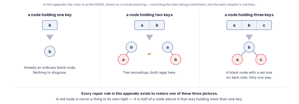
Read the rules off that picture rather than learning them. A red node is never a node in its own right; it is part of the black node directly above it, which is rule 4: a red whose parent is also red has no black node directly above it to belong to. Three keys together are a legal size, but the picture draws them one way only: a black node with a red child on each side. Counting black nodes down a path counts the 2-3-4 nodes on that path, and a 2-3-4 tree keeps all its leaves at one depth, which is rule 5, for free. The root is black because the top of a 2-3-4 tree is a whole node, which is rule 2.
And the middle column is the difference between this tree and LLRB, in one image. A two-key node has two legal drawings here, red on the left or red on the right, and the standard tree accepts both. LLRB forbids one of them. That is the entire disagreement between the two structures: the same idea, with a different amount of freedom, and every extra case in the standard tree’s code is the price of that freedom.
2.15.2 What the extra freedom costs
The two trees part company on real input. Hang 10, 20, 30, 15 into each, in that order. LLRB rotates at 10 and finishes with 15 on a black link holding 10 as its red left child. The standard tree finishes the other way round: 10 black, holding 15 as its red right child, a right-leaning red link, precisely the shape LLRB’s extra rule exists to forbid.
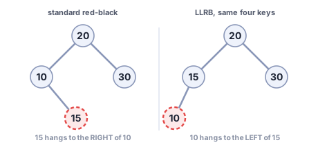
Same keys, same order, two different trees, both perfectly valid. Neither is wrong. They answer to a different number of rules.
What the freedom buys is worth naming, because it is the one place the standard tree is strictly ahead. Recoloring on either tree can climb all the way to the root. Rotations cannot: a single insert into the standard tree never needs more than two, and a single delete never more than three [5]. LLRB makes no such constant promise. If what you need is a hard bound on structural work per operation, and not merely on height, that is the reason to reach for the standard tree.
What the freedom costs is case-handling, and a good deal of it. Every extra shape the rules permit is another situation a repair has to recognize and another branch to get right. This book pays the other way, and said so when it chose: a slightly taller tree you can hold in your head.
The operations themselves are not developed here. They are in the standard references in full [2], [5], [12], and they will read as variations on moves you already have rather than as a new structure, which is the point of having derived this one from the same encoding.
That sentence is a claim, and you are in a position to test it. The next section is the test: the repair procedure is not printed anywhere in this book, and everything you need to reconstruct it is now behind you.
2.15.3 Derive the standard tree’s insert repair, without being told it
Exercise 35 · hardest in the chapter · ~120 min
You already have:
- the 2-3 tree behind LLRB, and why LLRB’s three moves are what they are
- the appendix’s encoding: a black node with its red children is one node of a 2-3-4 tree (black alone = 1 key, +1 red = 2 keys, +2 reds = 3 keys)
- the B-tree section, where you traced splits at minimum degree t = 2
The appendix states the standard tree’s five rules and stops. It does not give you its repair procedure. Derive it. Then say what the analogy was: which object mapped to which, and which move to which.
Three checks tell you whether you got it right:
- Predict, before running anything: which is more common on random keys, the split (the key lands in a full node) or the absorb (the node has room)? By roughly what ratio? Then measure it.
- Check your procedure against a real one. The companion library ships a standard red-black tree, built to the textbook rules rather than this chapter’s:
algodesign.searching.RBTree, inred_black_standard.py. Run your repair and its repair over the same keys and compare the trees node by node. This is the oracle, the reference you check against. If you disagree with it, one of you is wrong, and finding out which is the exercise. One kind of disagreement is not an error: if you split full nodes on the way down, as this chapter’s B-tree does, you have derived a different, also valid, member of the family. The next check is about exactly that. - Now the comparison that does NOT come out equal, and is the more interesting one. Build the same keys as a B-tree at t = 2, and group your red-black tree into its 2-3-4 nodes. Both are 2-3-4 trees on the same keys. They are often different 2-3-4 trees, though never on eight keys or fewer. Find the smallest key sequence where they differ, say what is still true of both, and explain the difference. It comes down to one line in the two procedures.
Then two questions:
- How many distinct routes reach this derivation? Find as many as you can, say what each one takes as given, and show they agree.
- Harder, and the real question. Every structure in this family keeps the same headline promise: the height stays within a constant factor of lg n, so search, insert and delete are all logarithmic. How many different sets of rules keep it? Not: how many ways to derive one set. How many sets are there, and what separates them?
Stretch: Now try deletion the same way. Fair warning: this one is harder and the analogy is looser. Say where it stops being an analogy.